| 1. | ||
| 2. | ||
| 3. | ||
| 4. | ||
| 5. | ||
Combined Method for Solution of Stefan Problem on Melting with the Account of Abrupt Change in Density
Khujaev J. I.
Center for the Development of Software and Hardware-Program Complexes, Tashkent University of Information Technologies, Tashkent, Uzbekistan
Email address
Citation
Khujaev J. I. Combined Method for Solution of Stefan Problem on Melting with the Account of Abrupt Change in Density. American Journal of Mathematical and Computational Sciences. Vol. 1, No. 1, 2016, pp. 10-17.
Abstract
A mathematical model of Stefan problem considering the density change during the melting process is proposed. The task is complicated by the fact that the boundary of the computational area becomes variable within the time. We offer a combined method for solving the problem with the use of numerical methods of catching the front and straightening the front. The results of computational experiments on melting ice and copper are given as example. Algorithms and software can be used to study the melting process of other pure substances.
Keywords
Stefan Problem, Heat Transfer, the Front of the Phase Transition, Melting, Numerical Method, Catching the Front, Straightening the Front
1. Introduction
Heat exchange processes associated with the change in the aggregate state of substance, are an integral part of many natural phenomena and technological processes. Melting of icebergs, evaporation of water from the ocean surface, storage technologies of various materials, including fruits and vegetables by freezing, defrosting and drying, thermal treatment of various materials, metal casting, and many others are examples of heat transfer processes related to the phase transition.
It is known that, during the change in the aggregate state, the physical parameters of the substance are subjected to changes. Along with the basic physical parameters such as thermal conductivity and heat capacity, also the density of the substance varies. Water freezing in a container forces it to expand, because when water freezes density decreases. So getting into the cracks of roads in winter, water freezes and expands the cracks and pits on the roads appear. On the contrary, in metals during the solidification, the density increases, and it decreases when they melt.
Heat transfer with phase transitions, the so-called Stefan type problems are always on the focus of researchers and scientists around the world. Developed various new and improved model based on the Stefan problem, taking into account abovementioned and other factors, are used in various fields of science and industry.
In his thesis, J. Back [1] considered the Stefan problem, for the study of melting processes of nanoparticles. The third chapter of the thesis discusses the problems of moving boundary that demonstrate the key properties of melting spherical substances, when the surface tension is taken into account. These problems are solved numerically using the finite difference methods. The fifth chapter discusses the two-phase Stefan problem for melting areas, taking into account the surface tension and kinetic undercooling. In this chapter, the model is considered in the context of the actual application of melting metal nanoparticles. In the models mentioned in the seventh chapter changes in the density and latent heat of fusion, depending on particle size are taken into account. When melting metal density decreases, the volume increases. This factor is considered in the models by adding an additional term in the heat equation governing the temperature of the liquid phase.
The problems of heat transfer and Stefan are studied in the work by M.R. Shabanova [2] based on the solution of non-local heat transfer equation in fractional derivatives with respect to time and coordinate. The first three chapters are devoted to the study of the current state of the mathematical theory of heat transfer, as well as the development of mathematical models of diffusion and convective heat transfer through the heat equation in fractional derivatives, subject to the initial conditions and without them. In the last chapter, a mathematical model of Stefan problem based on nonlocal heat equation is built. The results for various behaviors of phase boundaries respect to time and other parameters of derivatives of fractional order are obtained.
Various models on Stefan problems are discussed in PhD thesis by F. Font [3]. Chapters 2 and 3 investigate the melting processes of spherical nanoparticles, where the factor of abrupt change in density is considered. The fourth chapter describes the solidification models of supercooled liquids. In the fifth and sixth chapters of the thesis, the problems of energy saving in the Stefan problems are studied.
In his work, Sudakov I. A. [4] studied the interaction of the permafrost zone and the atmosphere, as a critical element of the climate system. The study is based on the hypothesis that under the influence of global warming, the melting of permafrost zones results in more greenhouse gas emissions, which have been accumulated inside the permafrost for a long time. The author developed a model for calculating the thermal state of permafrost zone based on the numerical scheme Patankara and conducted computational experiments. To predict the dynamics of melting process of permafrost lakes and methane emissions from permafrost zone nonlinear methods of theory of phase transitions based on the Stefan problem are used.
The article of V. R. Voller et al. [5] provides a solution of one-phase Stefan problems for melting. A special feature of the problem is the variable latent heat of melting, which increases linearly with increase of distance from the origin. This phenomenon can be attributed to the shoreline sedimentary basin motion model for tectonic inactivity period. The solution shows that the position of the shoreline has a dependency in the form of a square root function over time.
The article by S. H. Kim [6] proposes two simple numerical methods for finding the free boundary in a single-phase Stefan problem. The work is motivated by the need to improve the understanding of the solution surfaces (temperature) near the free boundary. The author has formulated logarithmically transformed functions with fixed and floating free boundaries, which have the Lipschitz character near the free boundary. To find a free boundary according to time a quadratic equation is solved recursively. Some numerical results are compared with the results from other methods.
An analytical solution of one- and two-phase Stefan problem is proposed in the article by J. Escher and others [7]. The existence of a unique smooth solution for a class of one- and two-phase Stefan problems with the correction of the Gibbs-Thomson in arbitrary spatial dimensions is proved. In addition, it is shown that the moving boundary depends analytically on the temporal and spatial variables.
The article of D. A. Tarzia [8] is devoted to the determination of expressions for one of the unknown thermal coefficients (such as thermal conductivity, mass density, specific heat and latent heat of melting) in a single phase fractional problem of Lamé-Clapeyron-Stefan. Using the latest results for the fractional diffusion equation and properties of Wright and Mainardi functions, necessary and sufficient conditions for the data to have a unique solution are found. Explicit expressions of the formulas are given in the form of a table.
The article by Rubtsov N. A. and others [9] is devoted to the study of processes of radiation-conductive heat transfer in semi-transparent media, such as, ice, glass, crystals, taking into account the phase transition. The authors propose a numerical model of a single-phase Stefan problem in a semitransparent layer with transparent boundaries that can partially absorb the radiation. By the results obtained, it can be said that the presence or absence of absorption of radiation within the boundaries affects the formation of the thermal field and a melting time. The paper argues that the absence of absorption slows down the heating and phase transition processes, and slight absorption in the boundaries greatly accelerates these processes as compared to the non-absorbent boundaries.
The principal methods of mathematical modeling of solidification and melting problems are analyzed in the article by Hu H. and Argyropoulos S. A. [10]. An analytical review of 100 references is presented. Different analytical methods that are used as standard assumptions to test numerical models are given. A set of mathematical formulations for the numerical solution of problems of solidification and melting are classified in the work. Based on a comprehensive review the main principles of choice of mathematical formulations to solve such problems are outlined.
Comparative analysis of several numerical methods for solving one-dimensional Stefan problems is given in the article of E. Javierre and others [11].
In the article of Lukyanov A. A. [12] the problem of melting of icebergs in the heat exchange with ocean water is reviewed. By using piecewise linear approximation the starting time of melting of ice is determined and a law of the movement of phase transition boundary (water-ice) is found.
The two-phase Stefan problem with a variable latent heat of melting, the initial temperature and constant heat flow is studied in the article of Salva N. N. and Tarzia D. A [13].
The usage of the phase change materials in the structure of composite materials of buildings (walls, floors, ceilings) is studied in the work by D. Heim [14] with the use of two methods in purpose of increasing the heat capacity of buildings.
The given above analytical review of the works on Stefan problem shows that the interest in these kinds of problems and their scope increases year by year. Of particular note are industries of environment, construction, development of composite materials, nanotechnology and others, the development of which directly related to the object of study of this work.
2. Statement and Mathematical Model of the Problem
We assume that a solid mass of material has a constant thickness ![]() and an initial starting temperature distribution
and an initial starting temperature distribution ![]() over the thickness. At a moment of time t=0, the body starts to heat up from
over the thickness. At a moment of time t=0, the body starts to heat up from ![]() with the variable temperature of
with the variable temperature of ![]() . If the density of the substance in a liquid state is higher than the density in the solid state, heating is carried out from the bottom of the body and vice versa. From the other end of the body, it is considered to be thermally insulated. To eliminate the abrupt temperature change, we accept the condition
. If the density of the substance in a liquid state is higher than the density in the solid state, heating is carried out from the bottom of the body and vice versa. From the other end of the body, it is considered to be thermally insulated. To eliminate the abrupt temperature change, we accept the condition ![]() , where
, where ![]() - the melting point of the material, which is assumed to be constant.
- the melting point of the material, which is assumed to be constant.
Under these assumptions, at time t=0, the front of phase change is formed, which corresponds to the initial coordinate of ![]() . A new zone - the liquid phase is formed. Denoting the temperature of the initial phase with
. A new zone - the liquid phase is formed. Denoting the temperature of the initial phase with ![]() , and a of new phase -
, and a of new phase - ![]() , let us build the heat transfer equations for both zones:
, let us build the heat transfer equations for both zones:
![]() , (1)
, (1)
![]() , (2)
, (2)
where the values of the coefficients of temperature conductivity are identified as ![]() and
and ![]() . Here
. Here ![]() ,
,![]() - densities of the substance before and after melting. Accordingly,
- densities of the substance before and after melting. Accordingly, ![]() and
and ![]() represent specific heat capacity,
represent specific heat capacity, ![]() and
and ![]() - thermal conductivity of the substance in the solid and liquid phases of matter. We neglect the changes of these parameters depending on the temperature.
- thermal conductivity of the substance in the solid and liquid phases of matter. We neglect the changes of these parameters depending on the temperature.
The initial state is in the solid phase:
![]() , (3)
, (3)
and actually a new phase is heated:
![]() . (4)
. (4)
and thermal insulation refers to a solid phase:
![]() . (5)
. (5)
The coordinate of the boundary between the phases ![]() is the phase transition front. Temperature at that boundary equals to the melting temperature
is the phase transition front. Temperature at that boundary equals to the melting temperature ![]() . Since the temperature doesn’t change when passing through the front, then we have the following condition:
. Since the temperature doesn’t change when passing through the front, then we have the following condition:
![]() . (6)
. (6)
Coordinate ![]() has a double meaning. On the one hand, it can be considered as the thickness
has a double meaning. On the one hand, it can be considered as the thickness ![]() of the already melted part of the initial phase. On the other hand, it may mean thickness of the newly formed phases. Since in the process of changing the state of aggregation the mass of the body remains unchanged, then for the unit area of the front of the phase transition we have an equation of
of the already melted part of the initial phase. On the other hand, it may mean thickness of the newly formed phases. Since in the process of changing the state of aggregation the mass of the body remains unchanged, then for the unit area of the front of the phase transition we have an equation of ![]() . In fact, the calculation of heat transfer is conducted through the thickness of the newly formed phase
. In fact, the calculation of heat transfer is conducted through the thickness of the newly formed phase ![]() by which conjugation condition of heat flux at the front of the phase transition can be written as
by which conjugation condition of heat flux at the front of the phase transition can be written as
![]() (7)
(7)
here L - latent melting energy, and ![]() - the speed of movement of the front of the liquid phase, while ensuring the continuity of medium.
- the speed of movement of the front of the liquid phase, while ensuring the continuity of medium.
This forms a difference ![]() in thicknesses. With the above assumptions, this difference leads to a movement of boundary of the computational domain to:
in thicknesses. With the above assumptions, this difference leads to a movement of boundary of the computational domain to:
![]() (8)
(8)
We shall therefore use the thickness of the newly formed phase and drop the index "2" in expressing. Then at the end of the melting process, when ![]() the coordinate of phase transition front and the thickness are equal to each other and are
the coordinate of phase transition front and the thickness are equal to each other and are ![]() :
: ![]() .
.
Note that when ![]() after melting the substance expands, when
after melting the substance expands, when ![]() - it shrinks. And when
- it shrinks. And when ![]() the volume remains constant and this case is mentioned in [15]. But in [15] the problem is solved for an infinite field (
the volume remains constant and this case is mentioned in [15]. But in [15] the problem is solved for an infinite field (![]() ) when the boundary conditions of the first kind are implemented.
) when the boundary conditions of the first kind are implemented.
Thus, the problem turns out to be with two unknown boundaries, although they are linearly dependent.
3. A Numerical Method for Solving the Problem
The presence of the moving boundary puts some restrictions to numerical methods, used to solve the problems with a constant boundary.
A method of catching front [16, 17] can be used for the initial stage of the melting process. This method consists of the search of time when the front of the phase transition reaches the calculation point with respect to x, in case the computational grid for x is constructed with a uniform step. Unfortunately, the final calculation point does not always coincide with the final thickness of the mass ![]() in case of moving boundary.
in case of moving boundary.
On the other hand, a method of straightening the front can only be applied when the front of the phase transition is located at a sufficient distance from boundaries [16]. Otherwise, an uncertainty associated with the division of ![]() and
and ![]() into small quantities is formed.
into small quantities is formed.
Based on the capability of these methods, we can divide the process of melting into three stages. In the first stage, we have implemented the method of catching front, in the second stage - a method of straightening the front, and the third stage is a linear extrapolation. The actual step on the coordinate x is h, and when ![]() , the method of catching front is used. The method of straightening the front is used until the conditions
, the method of catching front is used. The method of straightening the front is used until the conditions ![]() is satisfied.
is satisfied.
In implementing the method of finite differences [18] we have tried to ensure the accuracy of the second order of approximation with respect to x and time t.
In the method of catching front with the use of successive approximation we have determined the temperature fields and the value ![]() - the length of time during which the phase transition front moves from position
- the length of time during which the phase transition front moves from position ![]() to
to ![]() .
.
For a fixed value of n successive approximation is organized as follows.
For the zero-order approximation – ![]() we have determined the temperature field. According to the temperature field and with the involvement of the conditions of the energy balance at the front of the phase transition the next step approximation –
we have determined the temperature field. According to the temperature field and with the involvement of the conditions of the energy balance at the front of the phase transition the next step approximation – ![]() is determined. For this step of time the temperature field is found. On them we can determine
is determined. For this step of time the temperature field is found. On them we can determine ![]() . And etc. until the conditions of the temperature field are met according to
. And etc. until the conditions of the temperature field are met according to ![]() and the conditions of the energy balance at the front is satisfied.
and the conditions of the energy balance at the front is satisfied.
The internal points of the grid with a uniform step ![]() , where N – number of points in the input section due to time, for the s-th approximation for the heat transfer equation when
, where N – number of points in the input section due to time, for the s-th approximation for the heat transfer equation when ![]() we have approximated as:
we have approximated as:
![]() (9)
(9)
Multiplying both sides of the finite difference equation by ![]() and simplifying similar terms, we reached to a traditional form of the equation for sweeping:
and simplifying similar terms, we reached to a traditional form of the equation for sweeping:
![]() , (10)
, (10)
here ![]()
![]() .
.
Assuming that the values of coefficients ![]() of sweeping are known for the previous value of the index, we have found the values of sweeping coefficients for the present index:
of sweeping are known for the previous value of the index, we have found the values of sweeping coefficients for the present index:
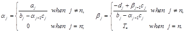 (11)
(11)
Such formulas are appropriate for forward sweeping of interior points of the zones of first (![]() ) and second (
) and second (![]() ) phases of matter with continuous numbering of the index j.
) phases of matter with continuous numbering of the index j.
As the starting point for calculating the values of coefficients of the sweeping served approximation equivalent of the conditions at x=0:
![]() . (12)
. (12)
Forward sweeping is carried out for ![]() .
.
For the calculation of the final point of ![]() the symmetry condition is approximated with the second order of accuracy:
the symmetry condition is approximated with the second order of accuracy:
![]() . (13)
. (13)
With the use of results of the direct sweep ![]() we find the temperature at the boundary:
we find the temperature at the boundary:
 (14)
(14)
Then the backward sweeping is carried out for ![]() according to the formula
according to the formula ![]() .
.
To determine the next step ![]() , we use the approximation of conjugation condition of the energy at the phase transition front in the form [16]
, we use the approximation of conjugation condition of the energy at the phase transition front in the form [16]
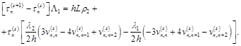 (15)
(15)
The value of the relaxation parameter ![]() is taken as equal to heat flux at the section of x=0:
is taken as equal to heat flux at the section of x=0:
![]() (16)
(16)
For n=1, the derivative of the temperature at x=0 in the last formulas were in the first order of approximation.
As the grid border Nl we took rounded to the nearest whole value of the expression ![]() .
.
Method of catching the front is implemented till it reaches the ![]() . Further we have used the method of straightening the front, for which as input parameters were:
. Further we have used the method of straightening the front, for which as input parameters were: ![]() and
and ![]() and the temperature distribution
and the temperature distribution ![]() – the result of the last step of the method of catching front.
– the result of the last step of the method of catching front.
In implementing the method of straightening the front the temperature field in the zone of a new phase is determined in the new coordinate of ![]() from the equation for the unknown
from the equation for the unknown ![]() :
:
![]() , (17)
, (17)
with the boundary conditions ![]() and
and ![]() .
.
For the zone of the initial phase temperature field is found with the new variable ![]() from the equation of
from the equation of ![]() and the boundary conditions
and the boundary conditions ![]() and
and ![]() .
.
Conjugation condition for the heat flow on the front of the phase transition (i.e. when ![]() ) takes the form:
) takes the form:
. (18)
The number of points on the input section when using the method of straightening the front is amounted at N1=64, N2=20. Hereinafter the values of steps in zones ![]() and
and ![]() are defined according to the values of N1 and N2. During solution process of the problem the values of N1 and N2 are changed automatically by the program, to ensure that the real values of the steps
are defined according to the values of N1 and N2. During solution process of the problem the values of N1 and N2 are changed automatically by the program, to ensure that the real values of the steps ![]() corresponding to them are in the interval of
corresponding to them are in the interval of ![]() .
.
A linear interpolation method [19] is used in the purposes of organization of the initial temperature distribution for the method of straightening the front, the preparation of the temperature field to save in order to visualize the results, as well as the transition to the step with another value on the coordinates.
For the i-th time section we have arranged successive approximation to determine the values of ![]() ,
, ![]() and the temperature in the zones of both phases. The next approximation of the temperature field is determined by the sweeping method, involving the previous values of
and the temperature in the zones of both phases. The next approximation of the temperature field is determined by the sweeping method, involving the previous values of ![]() and
and ![]() . To determine
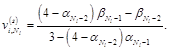
. To determine ![]() we have used the auxiliary formula
we have used the auxiliary formula
 (19)
(19)
In order to avoid the dynamic instability, as the last approximation in finding a new approximation we have used ![]() , and for the transition to the next section –
, and for the transition to the next section – ![]() .
.
This way of organizing the relaxation reduced the number of approximations of more than two times higher than using only ![]() .
.
4. Results and Discussion
The first series of calculations are performed for the process of melting ice. The followings are taken as input data:
c1=2.261103 J·kg-1·K-1, c2=4.618103 J·kg-1·K-1, λ1=2.250103 W·m-1·K-1,
λ2=0.4218103 W·m-1·K-1, L=3.335105 J·kg-1, ![]() ,
,![]()
The initial condition is taken as a ![]() , and the heating temperature in the section x=0 in the form
, and the heating temperature in the section x=0 in the form ![]() . Here, when
. Here, when ![]() the temperature has the value of
the temperature has the value of ![]() , then, increasing by the time
, then, increasing by the time ![]() it approaches to
it approaches to ![]() .
.
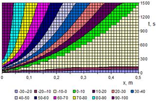
Fig. 1. The isotherms for ![]() , received at,
, received at, ![]() ,
, ![]() °C / m,
°C / m, ![]() m,
m, ![]() ,
, ![]() .
.
Fig. 1. shows the approximate isotherms at ![]() . As can be seen from the figure, the temperature fields are in the form of exponential lines. The temperature change occurs faster in the solid part of calculating area than in liquid part. We should notice that, the coefficient of temperature change a2 of ice is about 10 times higher than that of water. So the solid part is heated very fast and melting process begins. The front of phase transition is between the temperature fields of -10-0 (ivory) and 0-10 (green) and its form is like a stepwise function. In the liquid part the heat transfer occurs more slowly, as the slopes of lines become bigger.
. As can be seen from the figure, the temperature fields are in the form of exponential lines. The temperature change occurs faster in the solid part of calculating area than in liquid part. We should notice that, the coefficient of temperature change a2 of ice is about 10 times higher than that of water. So the solid part is heated very fast and melting process begins. The front of phase transition is between the temperature fields of -10-0 (ivory) and 0-10 (green) and its form is like a stepwise function. In the liquid part the heat transfer occurs more slowly, as the slopes of lines become bigger.
With the account of abrupt density change in melting, the length of the front of the phase transition is longer by about 10%: if ![]() the process with the account of the preliminary and final heat of the substance ended in the 2268 seconds, taking into account the variability of the boundary process is continued 2521 seconds (Fig. 2).
the process with the account of the preliminary and final heat of the substance ended in the 2268 seconds, taking into account the variability of the boundary process is continued 2521 seconds (Fig. 2).
During the melting process the density of ice increases and this fact causes the volume to decrease. This fact is seen in Fig. 2. as a decrease of the computational area (red dotted line).
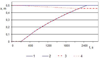
Fig. 2. The boundaries of the zone of the initial phase in the case of variable (dotted lines) and constant (solid line) boundaries for melting ice. Other data see. Fig. 1.
In addition, we have received the data on the complete melting of the ice with a thickness of 0.7 m: the time of the process continued 3517 seconds and 3970 seconds at variable and constant densities, respectively.
The comparison of the results for the duration of the melting process and consumed energy has shown that they are more than 10% less than in the case of ignoring the change in density during the phase change.
Water is a rare case of increasing the density of the material during melting. For metals the density tends to decrease during melting process. Next, we consider the results of numerical experiments regarding the melting process of a pure metall.
Computing experiments are carried out for melting process of copper. As initial data we have taken the followings:
с1=384.5 J·kg-1·K-1, с2=544.3 J·kg-1·K-1, Т*=1083°C, λ1=350.0 W·m-1·K-1 ,
λ2=250.0 W·m-1·K-1, ρ1=8940.00 kg·m–3, ρ2=8300.00 kg·m–3, L=212000 J·kg-1.
The values of the coefficients of heat transfer for copper in solid and liquid states are respectively ![]() and
and ![]() .
.
In this case, the ratio of the coefficients of heat transfer in solid and liquid states for copper is about two times. Therefore, the change in temperature on x coordinate will be smooth in the areas of both phases and there will be a small fracture on temperature curves at the front of the phase transition.
Keeping in common with the previous results, in the calculations we used excessive temperature relative to the melting temperature (1083°C). This has helped us to build visual materials, which show the melting front.
Calculations have been carried out for both changing and unchanging density cases.
Under these conditions, the duration of the initial heating (prior to the melting process) is 1260 seconds, which much longer than in melting ice (Fig. 3.).
Also we have checked the progress of successive approximation. In the fifth step of the method of catching front the number of repetitions is 39. The absolute difference between successive approximations ![]() after the 34-th approximation has been less than 10-8. Maximum absolute difference in the temperature field for two successive approximations has been less than 10-5 after 21-th approximation.
after the 34-th approximation has been less than 10-8. Maximum absolute difference in the temperature field for two successive approximations has been less than 10-5 after 21-th approximation.
The transition to the method of straightening the front occurred at t=1465 s. At t=1646, 2010 and 2216 seconds the value of the process step h1 of the first zone has been doubled. At t=1658 second and 2086 second the step of the second zone is reduced by half.
An exemplary process of successive approximation, according to the method of straightening the front is checked at t=1765 s. After the 14-th approximation all three conditions were satisfied. Besides, the accuracy of 10-7 is ensured in fulfilling the conditions of heat flux when passing through the phase transition front.
Fig. 3 shows the isotherms obtained for ![]() . The initial temperature of the body has a value of 30°C (in the calculations -1053°C), the asymptotic temperatures at x=0 is 1570°C (417°C in the calculations). The mass is heated according to exponential law
. The initial temperature of the body has a value of 30°C (in the calculations -1053°C), the asymptotic temperatures at x=0 is 1570°C (417°C in the calculations). The mass is heated according to exponential law ![]() .
.
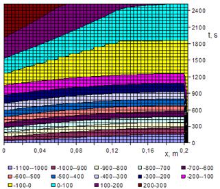
Fig. 3. The isotherms of process of melting the copper when ![]() , G=0.07159, τ=1.00 s, h=0.02 m,
, G=0.07159, τ=1.00 s, h=0.02 m, ![]() .
.
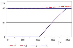
Fig. 4. Fronts of the phase transition and boundary of the computational domain at a constant (![]() m - solid lines) and variable (
m - solid lines) and variable (![]() – dashed lines) boundaries for melting copper.
– dashed lines) boundaries for melting copper.
Fig. 4. reflects the results for ![]() . When the boundary is variable the melting process ends at t=2427s, when the thickness is 0.21427 m, and at a constant boundary the time is 2326 s. The computational domain expands (red dashed line) as a result of density decrease in the process of melting copper.
. When the boundary is variable the melting process ends at t=2427s, when the thickness is 0.21427 m, and at a constant boundary the time is 2326 s. The computational domain expands (red dashed line) as a result of density decrease in the process of melting copper.
Thus, the opportunities of the developed mathematical model, numerical algorithms and software are tested for the cases of increase and decrease in the density of mass in the melting process.
5. Conclusions
In Stefan problem of melting two variants of forms of the front are identified: due to the initial phase and the newly formed phase. The difference between these coordinates appears as the change in boundary of calculation area.
The problem is formulated for the mixed types of boundary conditions (the first type at the beginning, the second type - at the end of the calculation region). The generalization of the mathematical model for other types of boundary conditions is also easy. You can also use other functions to describe the initial temperature distribution in the mass and the boundary condition at x=0, which would provide monotonous movement of front with respect to x axis.
By involving the method of catching front or straightening the front individually we cannot solve the problem, as the first method was developed to make calculations for the constant boundary of calculating range, and the second method cannot cover the cases of small phase thicknesses.
A numerical algorithm is developed for calculating the heat exchange process of the melting with the account of two unknown boundaries: the front of the phase transition and the boundary of calculating area. The combination of three methods; catching the front, straightening the front and successive approximation, is used with multiple changes in steps of the numerical integration of the equations.
To determine the phase transition front and unknown boundary of calculation range when using the methods of catching and straightening the front we have offered relaxation processes, which provide the necessary accuracy of calculation in the process of successive approximations.
To avoid the use of fractional steps, the boundary of the computational domain is rounded as multiple of the used step along x coordinate, it is permissible for small step numerical integration. Integration steps are automatically adjusted in the process of using both numerical methods, providing them to belong to the real interval.
The algorithm and the computer program developed on its basis are tested for the cases of increase and decrease in the density of matter during melting process. The obtained conclusive results demonstrate the real physical changes in the parameters of complex heat exchange process.
The given material (mathematical model, numerical algorithm and computer program) can also be successfully used in computer simulation of the solidification process, taking into account the density change of matter during the phase transition, in particular, the volume expansion of moisture during freezing which is often found in nature and technological processes.
References


