Design of a Rectangular Patch Microstrip Antenna 1.5 GHz for Global Positioning System (GPS)
Ossey Assi Agnissan Nicaise, Nene Franck Didier, Berenger Ouattara,
Kouassi N’goran, Fofana Siaka
Department of Signals and Systems, University of Felix Houphouet Boigny, Abidjan, Côte d'Ivoire
Email address

(O. A. A. Nicaise)

(N. F. Didier)

(B. Ouattara)

(K. N’goran)

(F. Siaka)
Citation
Ossey Assi Agnissan Nicaise, Nene Franck Didier, Berenger Ouattara, Kouassi N’goran, Fofana Siaka. Design of a Rectangular Patch Microstrip Antenna 1.5 GHz for Global Positioning System (GPS). Journal of Materials Sciences and Applications. Vol. 2, No. 2, 2016, pp. 18-24.
Abstract
This paper introduces the design of rectangular patch microstrip antenna with a frequency of 1.5 GHz that can be applied to the GPS antenna device. This antenna can improve the reception to GPS signals. The design of this antenna started with theoretical calculations then a simulation with the software MATLAB.
Keywords
Rectangular Patch Microstrip Antenna, GPS, MATLAB
1. Introduction
A microstrip consists of two words; they are micro (very thin / small) and strip (bar / piece). Microstrip antenna can be defined as one type of antenna that has the shape of blades / pieces that have a very thin size / small. Microstrip antenna consists of three parts; there are the patch, substrate, and ground plane. The patch is located on top of the substrate, while the ground plane is located at the very bottom. Once the microstrip circuit is fabricated, its adjustable factors are limited [1].
The deployment of the antenna technologies especially for government and commercial application such as mobile radio and wireless communications, an antenna that have requirements such as low profile, comfortable to planar and non planar surfaces, simple, inexpensive to manufacture using modern printed-circuit technology, ease of installation. Microstrip antennas meet these requirements. These antennas are very versatile in terms of resonant frequency, polarization, pattern, and impedance [2].
This microstrip can be used for small-needed-thing antenna such as for GPS. The incoming radio waves from GPS satellites undergo reflections, diffractions and scattering from buildings, trees, vehicles and other objects located in vicinity of the receiving antenna [3].
To take an advantage of GPS, we had to use the GPS receiver (GPS receiver). The task of the GPS signal receiver is looking for three or more of these satellites (by detecting signal emitted from the satellites), to determine the distance of each satellite from the receiver, and uses this information to determine the location of the observer who brought this receiver (based latitude and longitude). For information, the GPS signal transmitted in the L band frequency, i.e. the number 1575.42 MHz and 1227.60 MHz. The GPS receiving antenna pattern is necessarily hemispherical, further increasing its vulnerability to jamming [4].
2. Rectangular Patch
Microstrip antennas (often called patch antennas) are widely used in the microwave frequency region because of their simplicity and compatibility with printed-circuit technology, making them easy to manufacture either as stand-alone elements or as elements of arrays.
In its simplest form a microstrip antenna consists of a patch of metal, usually rectangular or circular (though other shapes are sometimes used) on top of a grounded substrate, as shown in Figure 1. [5]
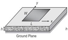
Figure 1. Microstrip rectangular patch antenna.
2.1. Determining Patch Settings
This part is to determine the electric parameters of the patch: the resistance, inductance, capacity and the supply inductance. All these parameters are a function of the resonant frequency and can be derived from each other. The antenna has the following characteristics: the length L, width W and height H. We first calculate the resonance frequency, the quality factor total QT then we will deduct the remaining parameters from [11], [12]:
 (1)
(1)
Where:
 is the position of the probe on the patch according to the axis x.
 (2)
(2)
With ωr = 2πfr
 (3)
(3)
 (4)
(4)
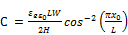
2.2. Resonance Frequency
Each patch is characterized by its effective length Leff and the effective width Weff which have minor effect on the resonant frequency. To make a rigorous calculation of we take into consideration these two parameters where the formula:
 (5)
(5)
With:
C0 = 3.108m/s.
m, n the number of mode.
For the calculation of the effective length, the following definition is used [11], [12]
 (6)
(6)
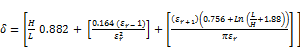
On the other hand, expressions of equivalent width Weq, and the effective permittivity εeff depending on width and length of the patch are given by the following equations
 (7)
(7)
 (8)
(8)
To calculate the coefficient Weq is used the impedance of a micro strip line as follows:
 (9)
(9)
It is found that, in calculating the effective width of the patch by replacing Weff Leff, L, Weq and Weff with W, Leq and L respectively include:
 (10)
(10)
 is the dynamic dielectric constant which is a function of the dimensions (W, L, H) and given by:
 (11)
(11)
Where:
 is the total dynamic capacity patch in the presence of air. Cdyn (ε) represents the total dynamic capacity patch in the presence of a dielectric of relative dielectric constant.
 (12)
(12)
The dynamic capacity Cody patch (ε) and dynamic marginal capacity Ce1 (ε) Ce2 (ε) are defined respectively as follows:
 (13)
(13)
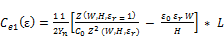 (14)
(14)
 (15)
(15)
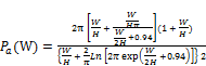
The characteristic impedance of the microstrip line Z (W, H, Er) is given by:
 (16)
(16)
if εr = 1 we have:
 (17)
(17)
Where the function f (X / H) is written:
 (18)
(18)
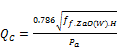
2.3. Calculation of Total Quality Factor
The total quality factor is expressed in terms of quality factors associated with radiation, conductor and dielectric loss by the following equation:
 (19)
(19)
With:
QR: the quality factor due to the radiation, is given by:
 (20)
(20)
Where εdyn is given by the formula (10).
Other contributions to the antenna quality factor is the loss of the dielectric and conductive. These losses are independent of the shape of the antenna if the substrate is thin.
 (21)
(21)
 (22)
(22)
With:
 (23)
(23)
tgδ: is the loss tangent of the dielectric given by:
 (24)
(24)
2.4. Feed Methods
Various methods may be used to feed the microstrip antenna, for the rectangular patch. We use the coaxial probe feed for this antenna shown in Figure 2
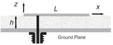
Figure 2. Feeding method for a microstrip antenna: coaxial feed [5].
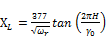
2.5. Input Impedance
Input impedance is defined as "the impedance presented by an antenna at its terminals or the ratio of the voltage to current at a pair of terminals or the ratio of the appropriate components of the electric to magnetic fields at a point."
The ratio of the voltage to current at these terminals, with no load attached, defines the impedance of the antenna as [2]
 (25)
(25)
Where:
 = antenna impedance at terminals
a-b (ohms)
 = antenna resistance at terminals
a-b (ohms)
 = antenna reactance at terminals
a-b (ohms)
In general the resistive part of (25) consists of two components; that is [2]
 (26)
(26)
Where
= radiation resistance of the antenna
 = loss resistance of the antenna
The radiation resistance will be considered in more detail in later chapters, and it will be illustrated with examples. [2].
If we assume that the antenna is attached to a generator with internal impedance [2]
 (27)
(27)
 (28)
(28)
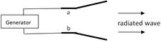
(a) Antenna in transmitting mode
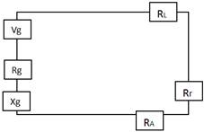
(b) Thevenin equivalent
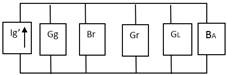
(c) Norton equivalent
Figure 3. Transmitting antenna and its equivalent circuits.
2.6. Radiation Pattern
Radiation Pattern Patch antenna’s radiation pattern shows that the antenna radiates more power in a certain direction than other directions. This characteristic in antennas is called directivity which is measured in dB. For an ideal patch antenna, all radiation is received in one half of the hemisphere which means 3dB directivity. In this scenario, all radiation is towards the front and no radiation is towards the back of the antenna. However, in real world applications, a portion of the radiation is towards the back of the antenna. The front to back ratio is very much contingent upon the size and shape of the ground plane. A patch antenna has a maximum directivity in the direction perpendicular to the patch. This directivity the antenna patterns (azimuth and elevation plane patterns) are frequently shown as plots in polar coordinates. This gives the viewer the ability to easily visualize how the antenna radiates in all directions as if the antenna was "aimed" or mounted already. Occasionally, it may be helpful to plot the antenna patterns in Cartesian (rectangular) coordinates, especially when there are several side decreases as the patch is moved towards the horizon. The 3 dB bandwidth is twice the angle of the maximum directivity. In another words, the 3dB bandwidth is where the directivity has dropped by 3dB; with respect to the maximum directivity.
2.7. Gain
The gain of an antenna (in any given direction) is defined as the ratio of the power gain in a given direction to the power gain of a reference antenna in the same direction. It is standard practice to use an isotropic radiator as the reference antenna in this definition. Note that an isotropic radiator would be lossless and that it would radiate its energy equally in all directions.
That means that the gain of an isotropic radiator is G = 1 (or 0 dB). It is customary to use the unit dBi (decibels relative to an isotropic radiator) for gain with respect to an isotropic radiator.
Gain expressed in dBi is computed using the following formula GdBi = 10*Log (GNumeric/GIsotropic) = 10*Log (GNumeric)
Occasionally, a theoretical dipole is used as the reference, so the unit dBd (decibels relative to a dipole) will be used to describe the gain with respect to a dipole. This unit tends to be used when referring to the gain of omnidirectional antennas of higher gain. In the case of these higher gain omnidirectional antennas, their gain in dBd would be an expression of their gain above 2.2 dBi. So if an antenna has a gain of 3 dBd it also has a gain of 5.2 dBi. Note that when a single number is stated for the gain of an antenna, it is assumed that this is the maximum gain (the gain in the direction of the maximum radiation). It is important to state that an antenna with gain doesn’t create radiated power. The antenna simply directs the way the radiated power is distributed relative to radiating the power equally in all directions and the gain is just a characterization of the way the power is radiated.
2.8. Polarization
The polarization or polarization state of an antenna is a somewhat difficult and involved concept. An antenna will generate an electromagnetic wave that varies in time as it travels through space. If a wave traveling "outward" varies "up and down" in time with the electric field always in one plane, that wave (or antenna) is said to be linearly polarized (vertically polarized since the variation is up and down rather than side to side). If that wave rotates or "spins" in time as it travels through space, the wave (or antenna) is said to be elliptically polarized. As a special case, if that wave spins out in a circular path, the wave (or antenna) is circularly polarized. This implies that certain antennas are sensitive to particular types of electromagnetic waves. The practical implication of this concept is that antennas with the same polarization provide the best transmission/reception path.
2.9. VSWR
The voltage standing wave ratio (VSWR) is defined as the ratio of the maximum voltage to the minimum voltage in a standing wave pattern. A standing wave is developed when power is reflected from a load. So the VSWR is a measure of how much power is delivered to a device as opposed to the amount of power that is reflected from the device. If the source and load impedance are the same, the VSWR is no reflected power. So the VSWR is also a measure of how closely the source and load impedance are matched. For most antennas in WLAN, it is a measure of how close the antenna is to a perfect 50 ohms.
3. Design Rectangular Patch for GPS Applications
This section discusses design of a rectangular patch with suitable bandwidth for GPS application. The bandwidth is defined as the frequency band in which VSWR is less that 2:1 which corresponds to -10 dB return loss i.e. the level at which 10% of the incident power is reflected back to source. The PATCH design parameters are Top radiating plate Length: 85mm, Width = 75 mm, ground plane is edge with side=120 mm, height (distance between ground and patch) = 6mm, Feed is vertical coaxial wire feed with wire diameter =0.2 mm. Air as dielectric, Figure 3 shows the PATCH for GPS applications and other Figures shows the MoM simulation results for the antenna.
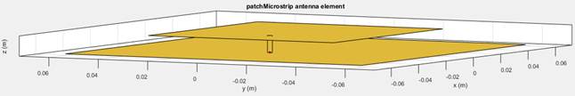
Figure 4. Design of a microstrip rectangular pacth antenna for GPS with Matlab 2015a.
4. Simulation Result and Analysis
These results are derived from simulation by MATLAB software:
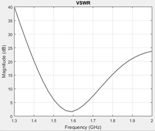
Figure 5. VSWR.
The best VSWR value is approaching a value of 1.2 and much of the value of VSWR=2 [6]. From the graph showed the smallest is worth 1:03 and at a frequency of 1,592 GHz.
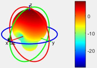
Figure 6. Gain.
The gain of the antenna is 8.48dBi Gain can be said to be good if the amount is more than 3dB.
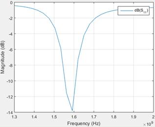
Figure 7. Return Loss.
From the graph known that return loss of microstrip antenna is below-10 dB jug shape, i.e. 90% of the signal can be absorbed, and 10% of reflected back. This return loss value is -13.82 [7], [8].
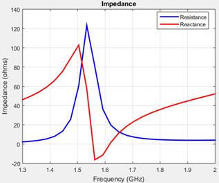
Figure 8. Input impedance.
Based on simulation results we select the two scenarios for the antenna integration with the chip. The antenna input resistance in the operational band varies from 36.35 Ohm till 123.2 Ohm, while the reactance varies from about -16.32 Ohm till 102.8 Ohm. Being differential fed by a source with 50Ohm output impedance the antenna operates (in terms of gain defined at 8.48 dBi level) from 1.5GHz till 1.6 GHz and exhibits a gain from -29.9 till 8.48 dBi.
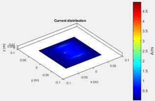
Figure 9. Current distribution.
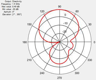
Figure 10. Radiation pattern with azimuth 0.
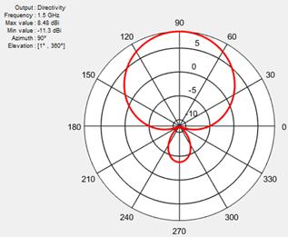
Figure 11. Radiation pattern with azimuth 90.
Results from Azimuth (polarization horizontal opening of the main lobe) at 90 degree is better than azimuth at 0 degree. The results of the simulation show that the antenna radiation pattern is isotropic [9].
The polarization results can be concluded that when the antenna is shifted vertically or horizontally not affect the power received [10].
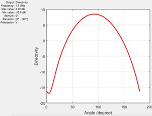
Figure 12. Vertical directivity with azimuth 0.
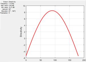
Figure 13. Horizontal directivity with azimuth 90.
5. Conclusion
From each result at these experiments, we can conclude that every single procedure whether in simulation or real measurements there will be always differences. It can be caused by materials or environment effects. For example, the differences of Gain and VSWR. The important gain of the antenna allows us to say that this antenna can help improve the reception of GPS signal. The antenna can be improved using slots in the patch or other sort of defected structures.
Acknowledgment
Thanks to ours teachers of university of Felix Houphouet Boigny (Deparment of signals and systems) for their supports.
Thanks for my family.
References
- Zhao Ying, Zhou Dong-fang, NiuZhong-xia, Zhang De-wei,"Study of the Influence of Resistors for Microstrip Equalizer" Institute of Information Engineering, Information Engineering University Zhengzhou 450002 China, APMC2005 Proceedings, 2005 IEEE.
- Balanis, Constantine A: Antenna Theory Analysis and Design Third Edition. John Willey and Sons, USA (2005).
- M. Dr Rehman, X. Chen, e.G. Parini and Z. Ying, "Effects of On-PCB Location of Radiating Element on the Performance of Mobile Terminal GPS Antennas in Multipath Environment", Queen Mary University of London, School of Electronic Engineering and Computer Science Mile End Road, London El 4NS (UK).
- B. Rama Rao, M. N. Solomon, M. D. Rhines, L. J. Teig, R. J. Davis, E. N. Rosario, "RESEARCH ON GPS ANTENNAS AT MITRE", The MITRE Corporation Bedford, Massachusetts 01730, 1998.
- John L. Volakis"Introduction and Fundamentals"of The Ohio State University.
- Tvrtko Mandic, Renaud Gillon, Bart Nauwelaersand Adrijan Baric,"Design and Modelling of IC Stripline Having Improved VSWR Performance", University of Zagreb, 2011.
- Parthakumar Deb, Tamasi Moyra and Priyansha Bhowmik, "Return Loss and Bandwidth Enhancement of Microstrip Antenna using Defected Ground Structure (DGS)", National Institute of Technology, Agartala, 2015.
- M. Arulaalan and L.Nithyanandan, "Return Loss Improvement in an Inset Fed Triangular Patch Antenna", International conference on Communication and Signal Processing, April 3-5, 2013, India.
- Vladimir Volski, Guy Vandenbosch, "Radiation Pattern Of a Microstrip Antenna Located on a Finite Size Ground Plane With Small Vertical Wall at the edges" KATHOLIEKE UNIVERSITEIT LEUVEN, 2001.
- S.-J. Shi and W.-P. Ding, "Radiation pattern reconfigurable microstrip antenna for WiMAX application" ELECTRONICS LETTERS 30th April 2015 Vol. 51 No. 9 pp. 662-664.
- F. Abboud, J.P. Damiano, and A. Papiernik, "Rectangular microstrip antenna for CAD,"IEEE Proceedings, Vol.135, Pt H, N°.5, pp. 323-326, October 1988.
- E. H. Newman, and P.Tylyathan, "Analysis of microstrip antennas using moment methods", IEEE Transaction on Antennas and Propagations, Vol. AP-29, N°. 1, pp. 47-53, Junuary 1989.


