Development of a Thermodynamic Modeling Framework (TMF) for Complex LNG Systems
Faith U. Babalola*, Oluwatosin S. Famoroti
Department of Chemical and Petroleum Engineering, University of Lagos, Akoka-Yaba, Lagos, Nigeria
Email address

(F. U. Babalola)

(O. S. Famoroti)
Citation
Faith U. Babalola, Oluwatosin S. Famoroti. Development of a Thermodynamic Modeling Framework (TMF) for Complex LNG Systems. Engineering and Technology. Vol. 3, No. 1, 2016, pp. 19-25.
Abstract
The Thermodynamic Modeling Framework (TMF) for LNG systems is obviously not available and its focal point is the development of robust methods for thermodynamic stability analysis as well as algorithms for accurate phase split predictions. A new model is here developed with its algorithm and applied to a Nitrogen-rich LNG system. Two EOS models were used with initial 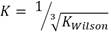 With Peng-Robinson EOS model, 2-phase split occurred at 110.8K, 3-phase–split occurred at 110.9K while the system reverted to 2 phases at 111K without further changes. For the Soave-Redlich-Kwong EOS model, the system split into 2 phases at110.8K, into 3 phases at 11K but reverted and remained a 2-phase system at 111.8K.
Keywords
LNG, TMF, Phase Stability, Phase Split
1. Introduction
In order to satisfy the energy demands of today’s modern society, the oil and gas industry focuses on the extraction, production, processing, transportation and storage of petroleum fluids. One of these important petroleum fluids can be conditioned into what is referred to as Liquefied Natural Gas. (LNG) Natural gas is generally considered a nonrenewable fossil fuel because most scientists believe that natural gas was formed from the remains of tiny sea animals and plants that died 200-400 million years ago.
Natural gas exists in nature under pressure in rock reservoirs in the earth’s crust, either in conjunction with and dissolved in heavier hydrocarbons and water or by itself. It is produced from the reservoirs similarly in conjunction with crude oil. Natural gas is used primarily as a fuel and as a raw material in the manufacturing industry.
Liquefied Natural Gas, (LNG) is natural gas in its liquid form. When natural gas is cooled to -259°F (-161°C), it becomes a clear, colorless, odorless liquid. LNG is neither corrosive nor toxic. Natural gas is primarily methane, with low concentrations of other hydrocarbons, water, carbon dioxide, nitrogen, oxygen and some sulphur compounds. Depending on the source of natural gas, its methane composition ranges between 87 and 99%. During the liquefaction process, natural gas is cooled below its boiling point
(-162°C) removing most of these compounds.
2. Lng Phase Behavior Modelling
The success of the design and operation of separation processes in the oil and gas
industry at cryogenic temperatures depends largely on the accurate descriptions of the thermodynamic properties and phase behavior of the concerned multi-component hydrocarbon mixtures with inorganic gases. Thus, it is important to develop a reliable thermodynamic modeling framework (TMF) that will be able to predict, describe and validate robustly and efficiently the complex phase behavior of LNG mixtures (Blanca et al., 2012). The TMF has three main components: a library of thermodynamic parameters pertaining to pure-substances and binary interactions, thermodynamic models for mixture properties and algorithms for solving the equilibrium relations. Reliable pure-component data for the main constituents of LNG systems are available experimentally the choice for the thermodynamic model is basically an Equation of State (EOS) Thus, the focal point of a TMF for phase behavior calculations of LNG systems is the development of robust methods for thermodynamic stability analyses, and of reliable efficient and effective flash routines for three phase split calculations. This work provides a robust method for carrying out thermodynamic stability analyses as well as flash routines for two- and three-phase split calculations. The model is here first demonstrated on an LNG sample.
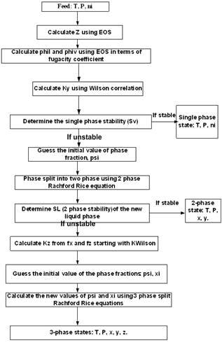
Figure 1. TMF Flow Chart for Complex LNG Systems.
3. Literature Review
Phase behavior relations have been explored in recent times by researchers for complex hydrocarbon systems (Adewunmi, 2014). Solution algorithms and new Equations of State have also been suggested for phase behavior calculations (Ayala, 2006; Dashtizadeh et al. 2006) Robust algorithms were suggested by Firoozabadi and Pan (2002) for stability analysis while Haugen et al (2011) developed robust three-phase split calculation methods. Isothermal flash calculation methods for multiphase systems were addressed by Naji (2008) and Rosales-Quintero (2009) while Iranshahr et al (2010) developed a generalized negative-flash method for similar systems. Three-phase split calculations using Rachford-Rice equation has been quite fruitful and promising as shown by Zhidong and Firoozabadi (2012a).
In this work, the stability testing criteria are explored and applied to three-phase split calculation using the Rachford-Rice rquation for a complex LNG system. The flow chart for the algorithm is shown in Figure 1.
4. Thermodynamic Stability Criteria
Stability testing has to do with knowing whether or not a mixture will actually split into two or more phases for a given pressure and temperature condition.
4.1. Single Phase Stability Testing
A single phase detection routine is used to detect whether the system is in a single phase condition at a given temperature and pressure or perhaps, it will actually split into two phases. Michelsen (1982a) suggested creating a second phase inside any given mixture to verify whether such a system is stable or not. The test must be performed in two parts considering two possibilities i.e. the second phase can be vapor-like or liquid-like.
4.2. Two Phase Stability Testing
The testing may be needed to know whether the mixture is stable in a given two-phase state. It is thermodynamically equal to testing the stability of one of the two equilibrium phases (Baker et al. 1982).
5. Phase Split Calculations
The majority of flash processes of industrial interest involve only a vapor phase and a single liquid phase. When it is known in advance that a given mixture at a specified pressure and temperature is incapable of forming multiple liquid phases it is fairly easy to decide whether a vapor-liquid phase split will occur (Michelsen, 1981b). A method for calculating the phase split for specifications in the two-phase and three-phase region is discussed.
Two-Phase Split Calculation.
Two phase Equilibrium satisfies the condition of equal fugacities of each component in both phases,  =
= (i=1 to C), where and are the fugacities of component i in phases x and y, respectively. The equality of fugacities can be further transformed using the natural logarithm of the equilibrium ratios as the primary variables (phase x is chosen as the reference) (Haugen et al. 2011) so that
 (i=1 to C) (1)
where  equilibrium ratio
 and
and  are the corresponding fugacity coefficients, but
  and
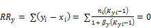
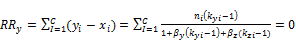
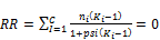
and  are restricted by the Rachford-Rice equation (Rachford and Rice 1952)
 (2)
(2)
Where  is the mole fraction of phase y. Eqn (1), Eqn (2) and , are used to carry out the two-phase equilibrium calculations. The phase compositions are determined from Eqms (3) and (4)
 (3)
(3)
 (i=1 to C) (4)
Three-Phase Split Calculations
Three-phase equilibrium satisfies the conditions (i=1 to C), where , and
  are the fugacities of component i in phases x, y and z, respectively. Similarly, the equilibrium condition can also be expressed in terms of the natural logarithm of the equilibrium ratios (phase x is chosen as the reference) (Haugen et al. 2011)
Establishing the three phases; V, L1 and L2, we have
 (5)
(5)
 (i=1 to C) (6)
for a mixture containing C components (Zhidong et al 2012) where and
and  are equilibrium ratios of component i with , and
  being the mole fractions of component i in phases x, y and z respectively,
  are the corresponding fugacity coefficients. The Rachford Rice equation is given by
 (7)
(7)
and
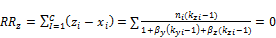 (8)
(8)
Where and  are the mole fractions of phase y and z respectively. Three-phase equilibrium is solved by combining Equations (7) and (8).
There are 2C+ 2 variables, { }, {
}, { }, and
  and the phase compositions are determined from
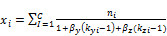 , (9)
, (9)
 , (10)
and
 (i=1 to C) (11)
6. The Procedure
(1) The Feed having composition ni under temperature T and pressure P is obtained.
(2) Calculation of Z using a selected Equation of State (EOS). Here two EOS are tested namely the SRK-EOS and the PR-EOS
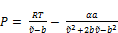
For Soave-Redlich-Kwong EOS
 (12)
(12)
where,
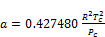
 (13)
(13)
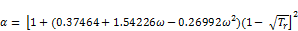
 (14)
(14)
 (15)
(15)
The SRK-EOS cubic expression in Z becomes:
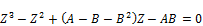 (16)
(16)
where
 (17)
(17)
 (18)
(18)
 (19)
(19)
 (20)
(20)
For Peng-Robinson EOS (Peng and Robinson; 1976)
 (21)
(21)
where:
 (22)
(22)
 (23)
(23)
 (24)
(24)
The PR-EOS cubic expression in Z becomes:
 (25)
(25)
where:
(26)
(27)
Similar to SRK-EOS, the PR-EOS mixing rules are:
(28)
(29)
(3) Calculation of phil and phiv using EOS, Z= roots (Arnulfo 2013)
Zl=minimum root of the cubic equation,
Zv=maximum root of the cubic equation
For SRK-EOS
 (30)
(30)
and for PR-EOS
 (31)
(31)
where
 (32)
(32)
 (33)
(33)
Phiv=exp(lnphiv) and phil=exp(lnphil)
(4) Calculation of Ky Using Wilson Correlation
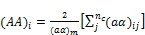
To calculate the mixture fugacity ( ) using overall composition ni
 (34)
(34)
Wilson’s correlation (Wilson; 1986) is used to obtain initial  values.
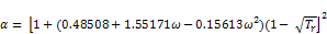
Wilson’s correlation and it’s reciprocal are used to provide the initial guess of { stab}. The Wilson correlation is given by
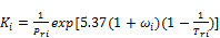 (35)
(35)
where  and
and  are the critical temperature, critical pressure, reduced temperature, reduced pressure and acentric factor of component i respectively. The second phase mole numbers,
  are calculated using
 (36)
(36)
To obtain the sum of the mole numbers,
 (37)
(37)
Normalizing the second phase mole numbers
 (38)
(38)
To calculate the second-phase fugacity () using the corresponding EOS and previous composition
 (39)
(39)
To calculate corrections for the k-values
 (40)
(40)
 (41)
(41)
(5) Single Phase Stability test is done; If Sv>1 the system is unstable otherwise it is stable and single phase condition prevails. 2-phase split calculation is next (if unstable)
(6) Initial Vapour Phase Fraction, Psi is Guessed
(7) 2-phase split calculation is done
 (42)
(42)
The phase compositions are determined from
 (43)
(43)
 (44)
(44)
 (i=1 to C) (45)
(8) Liquid phase fraction,  is calculated
calulated from Wilson’s correlation
(46)
 (47)
(47)
To calculate a liquid-like second phase
 (48)
(48)
 =∑
=∑ (49)
(49)
 (50)
(50)
 (51)
(51)
(52)
The system is stable if SL<1and if unstable SL>1
(9) Calculation of Kz is done
 (53)
(53)
(10) Initial values of the phase fractions: psi, xi. are guessed. Preferably, psi = its previous value from two-phase split RR equation while xi = 0 (Zhidong et al, 2012).
(11) Calculation of the new values of psi and xi using 3-phase split Rachford Rice equations Values of psi and xi are obtained by solving 3-phase Rachford Rice equations
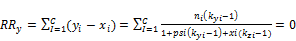 (54)
(54)
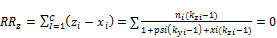 (55)
(55)
(12) 3-phase state properties; T, P, x, y, z are calculated.
There are 2C+ 2 variables, { },{
},{ }, psi and xi The phase compositions are determined from
 =
= , (56)
, (57)
(i=1 to C) (58)
The LNG system used for the model was sourced from Baltimore Gas and Electric LNG culled from liquid methane fuel characterization and safety assessment report Dec, 1993. Tables 1 and 2 show system parameters needed for the modeling. This LNG sample was deliberately selected due to its high nitrogen content which is above 1%.
Table 1. LNG Sample Parameters.
| Parameter | Value | Unit |
| R | 0.00008314 |  bar bar
|
| P | 1.013 | Bar |
| T | 111 | K |
Table 2. LNG Constituents and Their Properties.
| Component | Ni | Ω | | | Boiling Point |
| 
| 0.9332 | 0.0074 | 190.6 | 46.4068 | 111 |
| 
| 0.0465 | 0.0983 | 305.4 | 48.8385 | 187 |
| 
| 0.0084 | 0.1532 | 369.8 | 42.5666 | 231 |
| 
| 0.0018 | 0.2008 | 425.2 | 37.9662 | 273 |
| 
| 0.0101 | 0.0400 | 126.2 | 33.9437 | 77.21 |
7. Results
During simulation using our TMF, different number of phases were obtained as changes in T occurred.
7.1. Peng-Robinson (PR) EOS Model
Tables 3 and 4 show the values for PR EOS model using different K values as indicated

Tolerance = 
Table 3. Number of Phases Against Temperature.
| T (K) | 110 | 110.5 | 110.7 | 110.779 | 110.8 | 110.85 | 110.9 | 111 | 111.5 | 111.8 | 112.. | 115 | 120 |
| No Of Phases | 1 | 1 | 1 | 1 | 2 | 2 | 3 | 2 | 3 | 3 | 3 | 3 | 3 |

Tolerance =
Table 4. Number of Phases Against Temperature.
| T (K) | 110 | 110.5 | 110.7 | 110.779 | 110.8 | 110.85 | 110.9 | 111 | 111.5 | 111.8 | 112 | 115 | 120 |
| No Of Phases | 1 | 1 | 1 | 1 | 2 | 2 | 3 | 2 | 2 | 2 | 2 | 2 | 2 |
7.2. Soave- Redlich-Kwong (SRK) EOS Model
Tolerance =
Table 5. Number of Phases Against Temperature.
| T(K) | 110 | 110.5 | 110.7 | 110.779 | 110.8 | 110.85 | 110.9 | 111 | 111.5 | 111.8 | 112 | 115 | 120 |
| No Of Phases | 1 | 1 | 2 | 3 | 2 | 2 | 2 | 3 | 3 | 3 | 3 | 3 | 3 |
Tolerance =
Table 6. Number of Phases Against Temperature.
| T(K) | 110 | 110.5 | 110.7 | 110.779 | 110.8 | 110.85 | 110.9 | 111 | 111.5 | 111.8 | 112 | 115 | 120 |
| No Of Phases | 1 | 2 | 3 | 3 | 2 | 2 | 2 | 3 | 3 | 2 | 2 | 2 | 2 |
8. Discussion of Results
The algorithm developed for the Thermodynamic Model Framework (TMF) has deliberately included the following parameters: R,  ,
,  , ω, T, P, BIP and
  shown in Table 1 and Table 2. Some of the parameters generated are the
  ,
,  , Z, phi,
  ,
,  ,
,  , psi, xi, x, y and z. The programming code used for developing and executing the TMF was MATLAB.
Obviously, the program was able to generate reasonable results going by the output on Tables 3, 4, 5 and 6. Two popular Equations Of State- Peng-Robinson EOS and Soave-Redlich-Kwong EOS-were employed. Very critical in the modeling is the value of our K in arriving at reasonable results. could be initialized in various forms to obtain K-values which include: ,  .
. or
or  These provide the initial guesses for
  for stability testing (Zhidong et al, 2012).
 and
and  were selected as initial K values for the two-phase stability testing for both Equations of State.. The tolerance put at below is also a potent factor in order to obtain the results shown. All the values obtained are obviously the function of varying temperature at constant pressure. The pressure throughout is 1 atmosphere.
Peng- Robinson EOS Model
The results in Table 3 show that for initialized for two-phase stability testing, the LNG system is a single-phase liquid up till 110.779K after which at 110.8K it exhibited a two-phase characteristic which is V-L at 110.9K, then a three-phase system (V-L1-L2) was obtained and at 111K it returned to a two-phase system while at 111.5K it became three-phase again. The three phase system is retained till 120K, with no further changes.
Table 4 shows the results for the same system under the same condition only that our initialized K-values for two phase stability testing was . Just like for PR-EOS in Table 3, the system was a single-phase liquid at temperature values lower than 110.8K. Between 110.8K and 110.85K, a two-phase system (V-L) was obtained which turned to three phases (V-L1-L2) at 110.9K and becomes a two-phase system again at 111.5K and the two-phase system was maintained till 120K.
In effect, the two models predicted intermittent phase splitting and merging yielding one, two and three phases. Also at 110.9K both models generated the same result. But in practical terms, the result in Table 4 is more realistic than that in Table 3 since the constant three-phase system at 111.5K and beyond (in Table 3) may be impractical. Nitrogen in the system is expected to thin out as the temperature of the system increases and the third phase which is believed to be liquid phase nitrogen should disappear.
Soave-Redlich-Kwong EOS Model
In Table 5, the single-phase system ended at 110.5K and at 110.7K a two-phase system emerged. At 110.779K a three-phase system was obtained and at 110.8K a two-phase system was again observed. This continued until at 110.9K but at 111K the system became ternary in phase. The three-phase system was maintained until 120K.
As shown in Table 6, the system was one-phase (L) at 110K but split into two phases (L-V) at 110.5K. The binary phase system compounded to three-phase from110.7K until 110.779K after which it reverted back to two-phase till 110.9K. At 111K, a three-phase system was obtained again and remained untill 111.5K. Finally, a two-phase equilibrium system was gotten at 111.8K and was maintained until 120K.
It can be inferred from Tables 5 and 6 that the system under the influence of temperature exhibited phase split from one to two and from two to three phases and the reverse at some points. But the system is characterized by recurrence of specific equilibrium states. It is also obvious that Table 6 is more realistic than Table 5.
From the discussion so far, phase split in the LNG system has been successfully predicted as the system undergoes temperature variation using the TMF developed in this work. For phase split stability calculations, Kstability = is appropriate for both EOS medels. The results obtained were very close with a very small difference of about 0.57%. The same TMF can serve other purposes such as calculation of the composition of the different phases evolving from the feed as a function of the temperature of the system.
9. Conclusion
A robust TMF has been developed, tested, and its results analyzed. It is convincing that the model is workable and applicable to complex LNG systems. Hence the inverse cube root of Kwilson provides an appropriate guess in initializing Kstability for both EOS models used here. It can also be applied to any multi-phase fluid system. Phase split occurrences in a nitrogen-rich LNG system has been modeled. As far as the authors are aware, this TMF is novel and has not been built for complex LNG systems before.
References
- Blanca E. Garcia-Flores, Justo-Sarcia D. N., Stateva R. P., Garcia-Sanchez F. (2012) Phase Behaviour Prediction and Modelling of LNG Systems with Eoss- What is Easy and What is Difficult? Advances in Natural Gas Technology.ROUMIANA PETROVA STATEVA,vol. 14: 359-363.
- Adewumi A. (2014).PNG 520, Phase Relations in Reservoir Engineering-Phase Behaviour of Natural Gas.The College of Earth and Mineral Resources. The Pennsylvania State University,www.e-education.psu.edu/png520.
- Ayala, L. (2006). Phase Behaviour of Hydrocarbon Fluids –The Key to Understanding Oil and Gas EngineeringPetroleum and Natural Gas Engineering, the Pennsylvania State University.Business Briefing: Oil & Gas Proc. Review. 2006: 18.
- Dashtizadeh G., Pazuki G. R., Taghikhani V. and Ghotbi C. (2006) A New Cubic Equation of State for Predicting Phase Behavior of Hydrocarbons. Oil and Gas Science and Technology –Rev. IFP, Vol. 61, No. 2, 269-276.
- Firoozabadi A., SPE, and Pan H., SPE, (2002). Fast and Robust Algorithm for Compositional Modelling. Reservoir Engineering Research Institution, Part 1 - Stability Analysis Testing SPE Journal Vol. 7: 78, 79.
- Haugen K. B., Firoozabadi A,Kjetil B., Sun L. (2011). Efficient and Robust Three-Phase Split Computations. Chemical Engineering Dept., Mason Laboratory, Yale University, Reservoir Engineering Research Institute (RERI), 12452 Aiche Journal Vol. 57, No 9: 2555-2557.
- Naji H.S. (2008). Conventional and Rapid Flash Calculations for the Soave-Redlich-Kwong and Peng-Robinson Equations of State. King Abdulaziz University, Jeddah, Saudi Arabia.Emirates Journal for Engineering Research, 13 (3): 81-85.
- Rosales-QuinteroA. (2009)Isothermal Flash Calculation Using Soave Equation of StateMulticomponent Flash Calculations Using an Equation of State and Classical Mixing Rules.File ID: #22364, Version: 1.1 MATLAB CENTRAL1994-2013 The Mathworks, Inc.
- Iranshahr A., Voskov D., Tchelepi H.A. (2010). Generalized Negative-Flash Method for Multiphase Multicomponent Systems Department of Energy Resources Engineering, School of Earth Sciences, Stanford University, Elsevier B.V. Vol. 299, Issue 2: 272-274.
- Michelson, M. L. (1982a).The isothermal flash problem. Part I. Fluid Phase Equilibrium. 9 (1): 1-19.
- Baker, L. E. Pierce, A. C. and Luks, K. D (1982) Gibbs Energy Analysis of Phase Equilibria. SPE J 22 (5): 731-742. SPE-9806-PA.
- Michelson, M. L. (1982b).The isothermal flash problem. Part II. Phase split calculation. Fluid Phase Equilibrium. 9 (1):21-40.
- Haugen, K. B. Firoozabadi, A. and Sun, L. (2011). Efficient and robust three-phase split computations. AIChE J. 57(9): 2555-2565.
- Rachford, Jr, H. H. and Rice, J. D (1952). Procedure For Use Of Electronic Digital Computers In Calculating Flash Vapourization Hydrocarbon Equilibrium. Transactions of The American Institute of Mining and Metallurgical Engineers. Vol. 195. SPE 952327-G, 327-328.
- Zhidong Li, Abbas Firoozabadi (2012a) Initialization of phase fractions in Rachford–Rice equations for robust and efficient three-phase split calculation Reservoir Engineering Research Institute (RERI). Fluid Phase Equilibria 332 (2012) 21–27.
- Soave, G. (1972). Equilibrium constants from a modified Redlich-Kwong equation of state, Chem. Eng. Sci. 27: 1197- 1203.
- Peng, D. Y. and Robinson, D. B. (1976). A New Two-Constant Equation of State. Industrial and Engineering Chemistry Fundamentals (15): 59-64.
- Wilson, G. M. (1968). A Modified Redlkich-Kwong Equation of State, Application to General Physical Data Calculations. Presented at the 65th national AIChE meeting, Cleveland, Ohio, USA, 4-7 May, paper 15-C.
- Zhidong, L. and Firoozabadi, A.:(2012b) General Strategy for Stability Testing and Phase Split Calculations in Two and Three Phases. SPE, RERI and Yale University. SPE journal December 2012: 1-6.
- Introduction to LNG, Centre for Energy Economics. Liquid methane fuel characterization and safety assessment report. Cryogenic fuel Inc. CFI 1600, Dec. 1993: 17-20.


