An Improved Method for Crustal Temperatures: Implications for a Global Framework of Geotherms
Alexandrino C. H.1, Hamza V. M.2
1Federal University of the Jequitinhonha and Mucuri Valleys, Teófilo Otoni (MG), Brazil
2National Observatory, Rio de Janeiro (RJ), Brazil
Email address

(Alexandrino C. H.)

(Hamza V. M.)
Citation
Alexandrino C. H., Hamza V. M. An Improved Method for Crustal Temperatures: Implications for a Global Framework of Geotherms. International Journal of Geophysics and Geochemistry. Vol. 3, No. 6, 2016, pp. 61-72.
Abstract
An improved method for calculating crustal geotherms in stable continental crust is proposed, based on integrated use of data acquired in crustal seismic and heat flow studies. Designated as seismo-thermal method (STM), it is based on analytical solution to the standard heat conduction problem in stratified media, coupled with empirical relations between seismic velocities and temperatures at the crust-mantle interphase. Iterative trial and error methods are employed in establishing successful coupling. This technique allows estimation of crustal temperatures and mantle heat flow with lesser uncertainty than has so far been possible. The results obtained are relatively free of errors arising from the petrological complexities of the upper crust and are in broad agreement with crustal temperatures derived by conventional methods. Examples of the use of this method has been illustrated by calculating basal temperatures and crustal geotherms for four distinct segments of the Tocantins Structural Province in Brazil, namely the Araguaia Belt, Goiás Massif, Fold and Thrust Zones and Regions of sedimentary cover adjacent to the Sao Francisco Craton. The basal temperatures at the crust-mantle interphase in this province are found to fall in the interval of 760 to 1034°C, while the overall crustal thermal gradients are in the range of 16 to 20°C/km. Calculations of mantle heat flow, as per STM, indicate values in the range of 37 to 51mW/m2. The results reveal that deep crustal heat flow is relatively high in the Araguaia Belt and Goiás Massif, when compared with that in regions of Thrust and Fold Belts and sediment cover over São Francisco craton. Such second order changes in deep-level heat flow have not so far been detected in earlier studies based on conventional geothermal mapping. Use of the newly proposed method (STM) also opens up the possibility of setting up a global reference framework of deep geotherms in different tectonic settings, based on results of crustal seismic surveys.
Keywords
Crustal Geotherms, Seismo-thermal Method, Tocantins Structural Province, Seismic Velocities, Mantle Heat Flow, Global Framework for Geotherms
1. Introduction
Understanding the deep thermal field of crustal segments is a relatively complex problem that require not only availability of suitable observational data for outlining temperature gradients and heat flux at depths but also knowledge of geological structures and physical properties of the main subsurface layers. Geothermal measurements made in shallow boreholes provide information on near surface heat flux. Such data may be employed along with suitably selected crustal models in making inferences on deep crustal thermal conditions. This is the traditional approach and has been used widely in deriving crustal geotherms in many continental regions [1,2,3]. However, considerable uncertainties exist in results of such models. The main weakness of the conventional approach is that the results are essentially downward extrapolations of temperatures, based on near surface thermal gradients and heat flow. Such calculations are based on assumed values of thermal conductivity and radiogenic heat production for subsurface layers. In the absence of direct information, minor errors in such parameters may easily lead to substantial deviations in calculated values of basal temperatures and mantle heat flow.
The crux of this problem is the lack of a suitable boundary condition at the base of the crust that can constrain the solutions within reasonable bounds. In this context, it is useful to note that results of crustal seismic studies are capable of providing valuable complementary information on the physical characteristics of deep crustal structures. Of particular interest in this context are data on seismic velocities at the base of the crust, which are related to temperature changes at the crust mantle boundary. Empirical relations between seismic velocity and temperature have been addressed in several earlier studies in connection with determination of sub-lithospheric heat flow [4,5,6,7,8,9]. In addition, methods for estimating temperatures from seismic data at the base of the crust have been discussed [10,11,12]. However, the focus of such works has been on determination of differences in the crustal structure and composition. The possibility of developing solutions that couple the results of seismic surveys with geothermal studies have not been pursued in earlier works.
In the present work, estimates of temperatures derived from data on seismic velocities at the base of the crust are employed jointly with results of conventional heat flow studies in deriving crustal geotherms with a much larger degree of reliability than has been possible so far. Hence, this approach is referred to as the seismo–thermal method (STM). In the following sections, we examine the theoretical basis of this procedure and its limitations. STM was employed for understanding deep crustal heat flow variations in the main geologic units of the structural province of Tocantins, located in the central parts of the Brazilian highlands. Comparative analysis with results of conventional geothermal method points to reasonable agreement. We also discuss the implications of this method for setting up global reference frameworks for continental geotherms, based on results of crustal seismic surveys.
2. Crustal Geotherm with Specified Bottom-Boundary Temperature
Crustal geotherms are usually derived, based on solutions to one-dimensional heat conduction equation that satisfy known boundary conditions at the top surface [2, 3, 13, 14]. In case of layered media, the solutions must also take into account the values of thermal parameters in each layer. For n-layered media with subscripts indicating layer numbers the relations for temperature (T) and heat flux (q) are:
 (1a)
(1a)
 (1b)
(1b)
In the above equations n is the layer number, A the radiogenic heat production, D its scale factor and l the thermal conductivity.
Thermal models based on equations (1a) and (1b) has been used widely in deriving crustal geotherms in many continental regions [1,2,3]. The main weakness of this approach stems from the fact that observational data on model parameters (heat flow, thermal conductivity and heat production) are usually available only for the near surface layer. Use of estimated values for model parameters of deeper layers leads to considerable uncertainties in downward extrapolations of crustal temperatures.
Substantial reductions in such uncertainties can however be achieved by imposing suitable boundary conditions at the base of the crust. For example, results of deep crustal geophysical investigations, such as seismic, gravity, aeromagnetic or magneto-telluric studies may be used in obtaining independent estimates of basal temperatures. In such cases, the solution of the heat conduction equation for temperature and heat flux at the bottom of crust may be written as:
 (2a)
(2a)
 (2b)
(2b)
where the subscripts n-1 and b refer respectively to the top and bottom boundaries of the basal layer. Thus, TB represents the known basal temperature derived by the independent method and Tn-1 is the unknown temperature at the top of the lower crust. Its value is coupled to temperatures in the upper layers, specified in equations (1a) and (1b). The coupling between equations (2a) and (2b) with those of (1a) and (1b) require iterative adjustment of model parameters through trial and error methods. Such calculations can easily be implemented through standard worksheet operations.
A remarkable feature of this approach is that the use of basal temperatures inferred from deep crustal geophysical studies impose constraints on the possible limits of crustal geotherms, calculated using equations (1a) and (1b). In fact, the selection of model parameters that allow compatibility with specified basal temperature lead to considerable reduction of uncertainties in the crustal geotherm. The reason is that the procedure employed in derivation of basal temperature is relatively independent of the petrological complexities of crustal layers. In addition, there are indications [15,16,17] that independent estimates of bottom boundary temperatures lead to geotherms that are more reliable, when compared with those derived exclusively using assumed values of model parameters. In the present work, attention is focused on the possibility of using results of deep seismic studies in deriving independent estimates of the basal temperatures of the lower crust.
3. Principle of the Seismo-thermal Method
The variation of seismic velocity with temperature and pressure has been discussed in several of the earlier works. The relations proposed by [12,18,19] are based on differences in the values of in-situ seismic velocities with those measured in laboratory conditions. Hence, correction factors are necessary to account for the effects of temperature and pressure. It may be written as [12]:
 (3)
(3)
where VP (20°C, 100MPa) is the velocity of compressional wave in km/s at 20°C and at 100MPa pressure. VP (T, P) is velocity of compressional wave in km/s at temperature (T) and pressure (P). B (T, P) is the correction factor evaluated at temperature T and pressure P, both of which are functions of depth. The relation for B is [12]:
 (4)
(4)
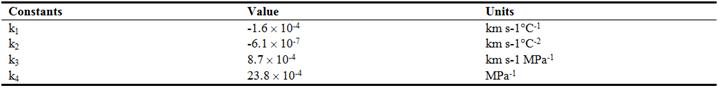
where k1, k2, k3 and k4 are constants and z the depth in kilometer. Figure 1 illustrates the nature of variation of the correction factor. The values of the constants adopted in the present work are given in Table 1. The correction factor is rather insensitive to small changes in the values of the constants.
The value of pressure in equation (4) may be obtained using the relation:
 (5)
(5)
where g is gravitational acceleration,  the density, and z the depth. The density for each layer may be estimated using the procedure described by [20].
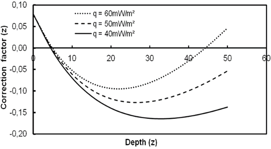
Figure 1. Variations in the value of the correction factor B(z) as a function of depth (Modified after [12].
Table 1. Representative values of the constants in equation – 4 (Modified after [12].
At this point, some comments on the effects of compositional changes on seismic velocities are in order. According to results of laboratory studies velocities of seismic waves depend not only on the ambient conditions of temperature and pressure but also on changes in the chemical composition of the medium. In fact, results of deep seismic investigations have revealed the existence of systematic trends in the relations between petrological characteristics and chemical compositions of crustal layers with vertical velocities of P and S waves (see for example, [20]). Geologic studies of uplifted blocks [21] indicate that compositional changes in the crust occur predominantly in the vertical direction and usually have spatial dimensions of less than a few kilometers [22]. In addition, composition of lower crust is in general mafic and uniform in different tectonic settings.
One of the consequences of compositional changes is that the values of the correction factor for seismic velocity (B) vary with the rock type. Nevertheless, changes in B values are found to be significant only in upper crustal layers, being much less pronounced within the lower crustal layer. According to interpretations based on results of global seismic surveys [20,23], the lower crust is composed predominantly of mafic rocks. In addition, the velocities have a strong dependence on the depth of the lower crustal layer, and are relatively independent of changes in rock types in the upper crustal layer. The absence of significant lateral variations of seismic velocities in deep crustal layers is indication that effects of compositional changes need to be considered only in special cases where crustal segregation processes have led to petrological inhomogeneity over distances large compared with the thickness of crustal layers. Since the application of STM is limited to estimates based on velocities in the relatively homogeneous lower crustal layer, the effects of compositional changes are unlikely to be major source of error.
4. Example of Application of STM
In the following sections, the procedure outlined above has been employed in calculating basal temperatures of the crust in the main geological units of the Tocantins structural province, in Central Brazil. Geological and tectonic framework of this region has been discussed extensively in several earlier works [24,25,26,27]. This area was selected in view of the availability of the results of two seismic refraction profiles, reported by [28,29,30].
The seismic profiles considered here cut across the main geologic units such as the Araguaia belt, Goiás Massif, regions of folds and thrust zones along the western parts of the Tocantins structural province as well as the rock sequences along the western border of the São Francisco craton. The western segment of the seismic profile (known as the Porangatu line) cuts across east central parts of this province. In the west, it starts over the Araguaia belt and then passes onto the northern part of the Brasilia belt, where the stations are situated over the units of Goiás Magmatic Arc, Goiás Massif and external basement zone. The eastern segment of the seismic profile (known as the Cavalcante line) cuts across the external zone of Brasilia Belt [28,29]. The locations of seismic profiles are indicated in Figure 2.
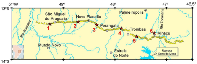
Figure 2. Location map of the seismic stations (yellow triangles). The shot points are indicated by the star symbols [28]. The inset map on the lower left corner indicates the location of the study area within the South American continent.
In follow up studies [29,30] reported mean values of longitudinal (Vp) and transverse (Vs) wave velocities of crustal layers for these geologic units. The results of seismic studies have allowed determination of the thicknesses of the crustal layers and values of density and velocities of primary (Vp) and secondary (Vs) seismic waves in the main crustal blocks of the Tocantins structural province. A brief summary of these results are reproduced in Table 2. With the exception of the top weathered layer, the P-wave velocities are in the range of 5 to 7 km s-1 while the S-wave velocities are in the range of 3 to 4 km s-1. The reported values of velocities have standard error of ± 0.05 km s-1.
The vertical distributions of S and P wave velocities are illustrated in Figure 3. As expected both P and S velocities increase rapidly with depth in the upper crust. This is followed by less pronounced increases in the middle and lower crustal layers. Another notable feature is the presence of low velocities at deep crustal levels in sediment-covered areas of the eastern parts, which is adjacent to the São Francisco craton (SFC). On the other hand, middle and upper crust beneath the Araguaia belt (AB) seem to be characterized by relatively high velocities. Intermediate values of velocities are found for crustal segments of Goiás Massif (GM) and regions of the thrust and fold belts (TFB). It appears that differences in velocities are more pronounced in the mid crustal levels relative to those in the lower crust. There are indications of a telescoping trend in velocities as the crust mantle boundary is approached. This is considered as indication that the lower crust of the study area is relatively uniform in composition and structure.
5. Basal Temperatures of the Crust in the Tocantins Province
Equations (3) and (4) have been employed, along with data on seismic velocities of Table 2, in determining basal temperatures and overall crustal thermal gradients of the main crustal blocks. The results obtained are presented in Table 3. Highest basal temperature of 1034°C was observed in areas of Araguaia Belt (AB). The lowest basal temperature was observed in regions of Thrust and Fold Belts (TFB). The Araguaia Belt (AB) and Goias Massif (GM) are found to have relatively high crustal thermal gradients (in the range of 22 - 23°C /km), followed by a slightly lower value of 18°C/km for the thrust and fold belts (TFB) of the Brasiliano orogenic belts. Lowest value of thermal gradient of 17°C/km was found for the region of sediment cover over the São Francisco Craton (SFC).
Table 2. Mean values of basal depths of layers and seismic velocities Vp and Vs for the main geologic units (Modified after [29]).
| Geologic Unit | Basal Depth (km) | Vp (km s-1) | Vs (km s-1) |
| São Francisco Cráton (SFC) | 0.1 | 3.6 | 2.0 |
| 1.4 | 5.7 | 3.3 |
| 12.4 | 6.1 | 3.4 |
| 30.3 | 6.2 | 3.6 |
| 47.6 | 7.0 | 4.0 |
| Thrust and fold belts (TFB) | 0.04 | 2.0 | 1.2 |
| 5.7 | 5.8 | 3.4 |
| 18.3 | 6.2 | 3.6 |
| 27.6 | 6.4 | 3.7 |
| 39.9 | 6.7 | 3.9 |
| Araguaia Belt (AB) | 0.1 | 2.0 | 1.2 |
| 2.1 | 5.8 | 3.4 |
| 12.4 | 6.2 | 3.5 |
| 19.7 | 6.6 | 3.8 |
| 35.4 | 6.9 | 3.9 |
| 44.7 | 7.1 | 4.1 |
| Goiás Massif (GM) | 0.1 | 3.3 | 1.3 |
| 3.8 | 5.9 | 3.4 |
| 14.1 | 6.2 | 3.5 |
| 22.3 | 6.4 | 3.7 |
| 40.1 | 6.8 | 3.9 |
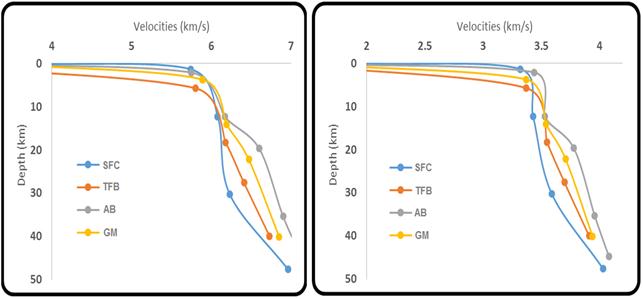
Figure 3. Vertical distributions of seismic wave velocities (Vp in the left panel and Vs in the right panel) in crustal segments of São Francisco Craton (SFC), Araguaia Belt (AB), region of Thrust and fold belts (TFB) and the Goiás Massif (GM).
Table 3. Basal temperatures and overall crustal thermal gradients calculated from seismic data for the main crustal segments of the Tocantins Structural Province.
| Geological Unit | Crustal Thickness (km) | Basal Temp. (ºC) | Overall thermal gradient (ºC/km) |
| Araguaia Belt (AB) | 44.7 | 1034 | 23 |
| Goiás Massif (GM) | 40.1 | 907 | 22 |
| Thrust and fold belts (TFB) | 42.8 | 808 | 18 |
| São Francisco Craton (SFC) | 47.6 | 825 | 17 |
6. Constraints on Crustal Thermal Field
Determination of reliable crustal thermal fields depend to a large extent on the success with which constraints can be imposed on the vertical distributions of thermal conductivity and radiogenic heat production in the deeper crustal layers. Observational data are, in general, available only for the upper crust. Errors in estimating values of parameters for deeper layers constitute a major source of uncertainty in calculations of crustal temperatures.
The procedure adopted in the present work minimizes this difficulty by imposing the condition that extrapolations of deep crustal temperatures converge to values obtained at the base of the crust from seismic data. In practice, estimates of basal temperatures of the crust (TB) in equations (2a) and (2b) are set to the values derived from equations (3) and (4). In the case of stratified media, adoption of this new procedure require use of a system of coupled equations for temperatures at the interphase between different crustal layers. In the scheme, illustrated in Figure 4, values of depth (z), radiogenic heat production (A) and thermal conductivity (l) are specified for each crustal layer. Thus, for an n-layered medium with subscripts indicating layer number, A0 and l0 represent values of the parameters at the surface (z = 0) and AB and lB represent values at the base of the crust (z = zB). Similarly T0 indicate temperature at the surface and TB that at the base of the crust.

Figure 4. Schematic representation of the layered model for heat production and thermal conductivity.
In the present work, crustal seismic data are also employed in obtaining estimates of vertical distributions of thermal conductivity and radiogenic heat production in crustal layers. Details of this procedure are presented in the following sections, with examples appropriate for the main geologic units in the Tocantins Structural Province.
6.1. Thermal Conductivity
The empirical relations proposed by [31] are often used as a guide in estimating the effects of pressure and compositional variations. In the present work, the pressure correction was performed using the expression:
 (6a)
(6a)
The values of δ adopted for the upper and for lower crust are 0.11 GPa−1 and 0.03GPa−1 respectively [32]. The effect of temperature (T) on thermal conductivity (l) has been accounted for by using the relation:
 (6b)
(6b)
In equation (6b), the coefficient l0, is the value of thermal conductivity at the reference temperature, and its value is determined by the relationship proposed by [33]. For the factor α we adopted the value proposed by [34] and for the factor β that proposed by [35]. The values adopted for α and β are respectively 10-3 and 5.0 x 10⁻¹⁰. A practical example of this procedure is illustrated in Figure 5 by considering the vertical distributions of thermal conductivity, derived from seismic velocity distributions in the four major crustal segments of the study area.
As can be verified, the calculated values of thermal conductivity are found to fall in the range of two to three W/m/K. Note that thermal conductivity decreases with depth in all crustal blocks, but there are no significant differences in values between crustal blocks at deeper levels. The right panel of this figure indicates the smoothed out trend of thermal conductivity in the crust.
6.2. Radiogenic Heat Production
Values of radiogenic heat production in crustal layers may be estimated using empirical relationships with seismic P wave velocities. The relation proposed by [36] has been widely used for geological formations of Paleozoic to Precambrian in age. More recently, [37] questioned the validity of such relations. Integrated analysis of the data sets by [36] and [37] has allowed [38] to propose a relationship that has been claimed to be independent of geologic age:
 (7)
(7)
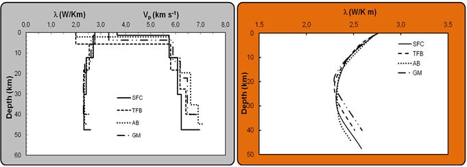
Figure 5. Vertical distributions of thermal conductivity (l) and crustal seismic velocities (Vp) in the crust in the study area. The right panel indicates the smoothed trends.
In the present work, use has been made of relation (7) in calculating values of radiogenic heat production for the main crustal layers. Figure 6 illustrate the vertical distributions of heat production derived from the seismic velocities, for the crustal segments of the Tocantins structural province. According to [39] near surface values of heat production vary from 1.18 μW m-3 in Goiás Massif (GM) to 1.55 μW m-3, in Fold Belts and Thrust Zones (TFB). At the lower crustal depths all crustal blocks have heat production values of less than 0.5 μW m-3. The smoothed trends of vertical variations in heat production are illustrated in the right panel of his figure.
In the absence of detailed information, it is usual practice to assume that the vertical variation of heat production in the crust can be approximated by exponential relations of the type:
 (8)
(8)
where A0 is the value of heat production at the surface (z = 0) and D the scale factor that governs the exponential decrease. A summary of the values of A0 and D, proposed by [39], are provided in Table 4 along with the respective standard deviations for the regions of the study area.
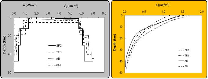
Figure 6. Vertical distribution of crustal seismic velocities (Vp) and heat production in crustal segments of the study area. The right panel indicates smoothed trends.
Table 4. Values of mean heat production (A0) and the scale factor (D) for the main crustal blocks in the study area (Adapted from [39]). The symbol s refer to values of standard deviation.
| Geological Units | Heat Production (μW m-3) | Scale Factor (km) |
| A0 | σA | D | sD |
| Araguaia Belt (AB) | 1.6 | 0.3 | 10.3 | 1.9 |
| Goiás Massif (GM) | 1.2 | 0.2 | 14.4 | 2.6 |
| São Francisco Cráton (SFC) | 1.4 | 0.3 | 13.6 | 2.4 |
| Thrust and fold belts (TFB) | 1.7 | 0.3 | 13.9 | 2.5 |
6.3. Near Surface Heat Flow
Results of heat flow measurements constitute the most important constraint in determination of crustal temperatures. The major difficulty however is in the availability of suitably deep boreholes for geothermal measurements. Over the last few decades, geothermal measurements have been carried out at nearly one hundred localities within the Tocantins structural province. Results of heat flow measurements for 16 localities was reported by [40]. More recently, [3,39,41] reported temperature gradient and heat flow values for additional 54 sites in the regions of Tocantins province and also in the São Francisco craton. A brief summary of the results of temperature gradients (Γ), thermal conductivity (λ) and near surface heat flow (q) for sites near the seismic survey belt is presented in Table 5.
Note that geothermal gradients and heat flow are relatively high in the Araguaia Belt (AB) and in the Goias Massif (GM), relative to those of Fold and Thrust Belts (TFB) and adjacent areas of the Sao Francisco Craton (SFC).
Table 5. Summary of geothermal data compiled for the Tocantins structural province.
(Γ is geothermal gradient, λ is thermal conductivity and q the near surface heat flow)
| Geologic Unit | Γ (C/km) | λ (W/m/K) | q (mW/m2) |
| Araguaia Belt | 25.2 | 2.7 | 68 +/- 23 |
| Goiás Massif | 23.8 | 2.7 | 64 +/- 14 |
| Fold and Thrust Belts (TFB) | 20.2 | 2.6 | 53 +/- 15 |
| São Francisco Craton (SFC) | 20.4 | 2.8 | 57 +/- 26 |
7. Crustal Geotherms in Tocantins Province
In deriving crustal geotherms, it is usual practice to make assumptions as to the vertical distributions of thermal conductivity, radiogenic heat production and surface heat flow. This is the common approach widely used in geothermal research, designated here as the conventional geothermal method - CGM. In the seismo-thermal method (STM) of the present work, an additional constraint is imposed according to which the calculated geotherms must also fit the basal temperatures derived from crustal seismic data. In other words, geotherms based on CGM need to satisfy only the top boundary condition while those based on STM must satisfy both the top and bottom boundary conditions. Clearly, there is a need to distinguish geotherms based on the seismo-thermal method (STM) from the ones based on the conventional method (CGM). However, derivation of geotherm based on STM require some minor adjustments in the values of the model parameters. Results of numerical simulations reveal that small changes in the values of surface heat flow, with magnitudes less than one standard deviation of the mean, are usually sufficient to bring about the fits. In practice, the value of surface heat flow is considered as a free parameter during the iteration process in obtaining physically reasonable fits with the basal temperature.
As an example, consider the vertical variations of temperatures and heat flow for the Araguaia Belt (AB), based on STM and CGM, illustrated in Figure 7. The left panel of this figure indicate vertical distributions of temperatures while the right panel indicate the same for heat flow. The continuous lines indicate geotherms by STM while the dashed lines indicate those by CGM. Geotherms by STM are characterized by systematically lower temperatures and heat flow relative to those for CGM. In both cases, there are substantial reductions in heat flow with depth in the crust. Though not illustrated in this figure, the general trends of geothermal gradients are similar to those found for heat flow. The basal temperatures by STM and CGM are respectively 1034 and 1038°C. There are indications that the differences between the two geotherms increase with depth in the crust.

Figure 7. Crustal geotherms for the Araguaia Belt (AB) by STM and CGM. The left panel indicates the vertical distribution of temperatures in the crust, while the right panel the vertical distribution of heat flow.
Similar results obtained for the region of Goiás Massif (GM) are illustrated in Figure 8. In this case however, geotherms by STM are found to have higher values relative to those for CGM. The results for Fold and Thrust Zones (TFB) and sedimentary cover of São Francisco Craton (SFC), illustrated respectively in Figures (9) and (10), are found to have trends similar to those of Araguaia Belt.
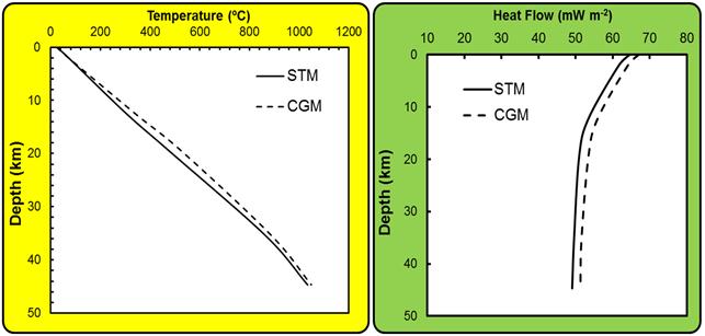
Figure 8. Crustal geotherms of the region of Goiás Massif (GM). The legends for the panels are the same as that in Figure (7).
It is useful to compare the results obtained by STM of the present work with those of the conventional geothermal method (CGM). In this context, we have selected results of conventional heat flow measurements made at sites close to the seismic reflection profiles of [29]. Most of these sites are located in regions of Goiás Massif (GM) and the Thrust and Fold Belts (TFB). Comparative results for surface heat flow and geothermal gradient obtained by the two methods are given in Table 6. It is important to point out that the results of Table 6 are means of site values and should not be confused with regional means given in Table 5. Note that there is reasonably good agreement between results obtained by the two methods. The values obtained by STM fall within the range of values calculated by CGM.
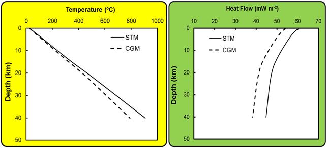
Figure 9. Crustal geotherms of the region of Thrust and Fold Belts TFB). The legend for the panels is the same as that in Figure (7).
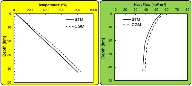
Figure 10. Crustal geotherms for the region of sedimentary cover over the western border of the São Francisco craton (SFC) by STM and CGM. The legend for the panels is the same as that in Figure (7).
Table 6. Comparison of the results obtained for near surface values of geothermal gradient and heat flow by CGM and STM.
| Crustal Block | Thermal Gradient (C/km) | Heat flow (mW/m2) |
| STM | CGM | STM | CGM |
| Araguaia Belt (AB) | 23.7±5 | 24.6±6 | 65±3 | 67±6 |
| Goiás Massif (GM) | 22.2±4 | 19.9±7 | 60±4 | 54±7 |
| Thrust and Fold Belts (TFB) | 20.2±3 | 20.9±8 | 55±5 | 57±9 |
| São Francisco Craton (SFC) | 20.4±3 | 21.6±5 | 56±6 | 59±8 |
A similar comparison have also been made for values of mantle heat flow and basal temperatures of the main crustal blocks. The results are presented in Table 7. As in the previous case, there is reasonably good agreement between results obtained by the two methods. The values obtained by CGM fall within the range of values calculated by the STM method. This is important as it shows the feasibility of using the results of crustal seismic studies as a complementary tool in geothermal investigations.
Table 7. Crustal thickness (zB), heat flow (qB) and temperatures (TB) in the four main crustal blocks of the base crustal for study area.
| Crustal Block | zB (km) | qB (mW m-2) | TB (C) |
| STM | CGM | STM | CGM |
| Araguaia Belt (AB) | 44.7 | 49±6 | 51 | 1034±20 | 1041±40 |
| Goiás Massif (GM) | 40.1 | 45±6 | 38 | 907±15 | 792±30 |
| Thrust & Fold Belts (TFB) | 39.9 | 37±6 | 39 | 808±15 | 849±30 |
| São Francisco Craton (SFC) | 47.6 | 35±6 | 41 | 825±15 | 892±30 |
8. Implications for Global Reference Frameworks of Geotherms
An important application of STM is the possibility of using results of crustal seismic surveys in setting up a global reference framework of deep geotherms in different tectonic settings. By reference framework for geotherms, we mean a system where the technique employed for calculating basal temperatures have a common basis, allowing for easy comparison of the results. Earlier attempts in setting up reference systems for crustal geotherms have met with only partial success because of the absence of a common framework for calculations of basal temperatures. This drawback stems from the fact that petrological complexities of the upper crust contributes to uncertainties in the model parameters employed in calculating crustal geotherms by the conventional methods. In STM, the procedure employed for calculating basal temperatures makes use of seismic velocities of the lower crust, in addition to information on surface heat flow. The technique used in measurement of seismic velocities is independent of the characteristics of the upper crust. According to results of geophysical and geochemical studies (see for example [42,43,44]) petrological complexities of lower crust are less severe when compared with those of the upper crust. In addition, it is present in a wide variety of tectonic settings and the procedure can be applied to any region with availability of suitable crustal seismic survey data.
The relatively uniform chemical composition of the lower crust in many continental regions means that the system of deep temperatures may be suitable for reference purposes on a global scale. This in turn should allow derivation of global maps of crustal geotherms with a common reference basis that is relatively free of the high frequency variations arising from geological complexities of upper crustal layers. The main obstacle in implementing STM is the lack of integrated geophysical studies in different tectonic settings, capable of setting reasonable bounds on deep crustal temperatures. In the present work, the procedure adopted in calculation of crustal geotherms are based on estimates of basal temperatures of the crust beneath the Variscan structural element in the northwestern Mediterranean [12,18,45]. Integrated analysis of data acquired in deep crustal geophysical investigations in other tectonic settings may allow for improvements in calibration of the proposed method.
It is clear that STM is helpful in understanding the relations between seismic velocities and crustal geotherms in different tectonic settings. The left panel of Figure 11 illustrates the nature of relation between surface heat flow and basal temperatures in the Tocantins structural province in central Brazil. The orange colored dots in the right panel of this figure indicates global distribution of localities where deep crustal seismic surveys have been carried out [46]. However, details of relations between basal temperature and heat flow remain unknown in many localities of deep seismic surveys, indicated in the right panel of this figure.
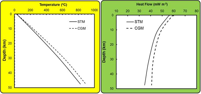
Figure 11. Left panel illustrates the nature of relation between surface heat flow and basal temperatures in the Tocantins structural province, Brazil. The right panel indicates global distribution of localities (orange colored dots - continental; blue dots - oceanic) with deep crustal seismic surveys (USGS, 2016).
9. Conclusions
The seismo-thermal method (STM) proposed in the present work makes use of analytical solutions to the heat conduction problem in stratified media, with coupling between results of seismic and geothermal studies. The boundary conditions imposed on temperatures in the lower crust and surface heat flow in the upper crust has allowed derivation of crustal geotherms with much lesser degree of uncertainty than can be achieved by conventional geothermal methods. This technique also allow determination of mantle heat flow compatible with estimates of vertical distributions of thermal conductivity and radiogenic heat production of crustal layers.
The method has been used in obtaining new insights into the thermal structure of the crust in the Tocantins Structural Province. Specifically, crustal geotherms, with much lesser degree of uncertainty, have been derived for the main crustal segments of the study area: Araguaia Belt, Goiás Massif, Fold and Thrust Zones and Regions of sedimentary cover adjacent to the São Francisco Craton. Basal temperatures at the crust-mantle interphase in the Tocantins structural province are found to fall in the interval of 760 to 1034°C, while the sub-crustal heat flow values fall in the range of 37 to 51mW m-2. The results reveal that deep crustal heat flow is relatively high in regions of Araguaia Belt and Goiás Massif, when compared with Thrust and Fold Belts of the Tocantins Province and regions of sedimentary cover of the adjacent São Francisco Craton. Such changes in deep-seated heat flow are found to be different from the trends observed in heat flow maps derived from results of conventional geothermal studies. We conclude that seismo-thermal method provides a new perspective for understanding the deep thermal structure of the crust in stable continental regions.
It also opens up the possibility of using results of crustal seismic surveys in setting up a global reference framework of deep geotherms in different tectonic settings [46]. In principle, the STM may also be employed for determination of basal temperatures in regions of oceanic crust. In this case, however, lack of resolution of seismic data is major problem and corrections for compositional variations need to be incorporated [47].
Acknowledgements
The present work received financial support of the National Council for Scientific Research in Brazil – CNPq, through grant n° 487501/2012-8 – APQ.
References
- Blackwell, D. D., 1971. The thermal structure of the continental crust: In: Heacock, J. G., (Ed.), The structure and physical properties of the Earth's crust: American Geophysical Union Monograph, 14: 169-184.
- Hamza, V. M., 1982. Thermal structure of the South American continental lithosphere during Archean and Proterozoic. Revista Brasileira de Geociencias 12: 149-159.
- Alexandrino, C. H., 2008. Thermal field of the structural province of São Francisco and adjacent mobile belts (in Portuguese), Unpublished Ph.D. Thesis, National Observatory (ON - MCTI), Rio de Janeiro, 183 pages.
- Kern, H., Richter, A. 1981. Temperature derivatives of compressional and shear wave velocities in crustal and mantle rocks at 6 kbar confining pressure. J. Geophys., 49: 47–56.
- Goes, S., R., Govers, Vacher, P., 2000. Shallow mantle temperatures under Europe from P and S wave tomography. J. Geophys. Res., 105: 11,153–11,169.
- Shapiro, N. M., Ritzwoller, M. H., 2004. Thermodynamic constraints on seismic inversions. Geophys, J. Int., 157: 1175–1188.
- Kuskov, O. L., Kronrod, V. A., 2007. Modelling of the thermal structure of continental lithosphere. Izvestiya, Physics of the Solid Earth, 43: 91–101.
- Perry, H. K. C., Jaupart, C., Mareschal, J.-C., Shapiro N. M., 2006. Upper mantle velocity-temperature conversion and composition determined from seismic refraction and heat flow. J. Geophys. Res., 111: B07301, doi:10.1029/2005JB003921.
- Vedanti, N., Pandey, O. P., Srivastava, R. P., Mandal, P., Kumar, S., and Dimri, V. P., 2011. Predicting heat flow in the 2001 Bhuj earthquake (Mw=7.7) region of Kutch (Western India), using an inverse recurrence method. Nonlinear Processes in Geophysics, 18: 611-625, doi:10.5194/npg-18-611-625.
- Cermák, V., 1982. Crustal temperature and mantle heat flow in Europe. In: M. L. Gupta (Editor). Terrestrial Heat Flow. Tectonophysics, 83: 123-142.
- Kern H, Schenk V (1988) A model of velocity structure beneath Calabria, southern Italy, based on laboratory data. Earth and Planetary Science Letters, 87: 325–337.
- Verdoya, M., Pasquale, V., Chiozzi, P., Kukkonen, I. T., 1998. Radiogenic heat production in the Variscan crust: new determinations and distribution models in Corsica (northwestern Mediterranean). Tectonophysics, 291: 63-75.
- Carslaw, H. S., Jaeger, J. C., 1959. Conduction of Heat in Solids, 2nd ed. Oxford: Oxford University Press.
- Özisik, M. N., 1980. Heat Conduction, John Wiley, New York.
- Artemieva, I. M., Mooney W. D., 2001. Thermal structure and evolution of Precambrian lithosphere: A global study. J. Geophys. Res., 106: 16387-16414.
- Spichak, V., Zakharova, O., Rybin, A., 2007a. On the possibility of realization of contact-free electromagnetic geothermometer, Doklady Russian Academy of Sci. 417A (9): 1370-1374.
- Spichak, V., Zakharova, O., Rybin, A., 2007b. Estimation of the sub-surface temperature by means of magnetotelluric sounding. Expanded Abstract. XXXII Workshop on Geothermal Reservoir Engineering, Stanford University, USA.
- Pasquale, V., Cabella, C., Verdoya, M., 1990. Deep temperatures and lithospheric thickness along the European Geotraverse. Tectonophysics, 176: 1-11.
- Cermák, V., Bodri, L., Rybach, L., 1991. Radioactive heat production in the continental crust and its depth dependence. In: Cermák, V., Rybach, L. (Eds.), Terrestrial Heat-Flow and Lithosphere Structure. Springer, Berlin, pp. 23-69.
- Christensen, N. I., and Mooney, W. D., 1995. Seismic velocity structure and composition of the continental crust: A global view, J. Geophys. Res., 100: 9761-9788.
- Zhai, M. –G, Guo, J. H. and Liu, W. –J., 2001, An exposed cross-section of early Precambrian continental lower crust in North China Craton., Physics and Chemistry of the Earth, 26: 9-10, 781-792.
- Caggianelli, A., Prosser, G., Festa, V., Langone, A., Spiess, R., 2013, From the upper to the lower continental crust exposed in Calabria., 86° Congresso Nazionale della Società Geologica Italiana-Arcavacata di Rende (CS), vol. 5 (1-2), 49p., DOI: 10.3301/GFT.2013.02
- Rudnick, R. L., Fountain, D., M., 1995. Nature and composition of the continental crust - a lower crustal perspective, Reviews in Geophysics 33: 267-309.
- Almeida, F. F. M., Hasui, Y., Brito Neves, B. B., Fuck, R. A., 1981. Brazilian structural provinces: an introduction, Earth Sciences Review, 17: 1-29.
- Fuck, R., A., 1994. The Brasilia Belt and tectonic partition in the Tocantins Province (in Portuguese). Proceedings of the Symposium in Brasilia on Geology of West-Central region, 4: 184-187.
- Pimentel, M. M., Fuck, R, A., Jost, H., Ferreira Filho, C. F., Araújo, S., M., 2000. The basement of the Brasília Fold Belt and the Goiás Magmatic Arc, In: Cordani, U. G., Milani, E., J., Thomaz Filho, A. and Campos, D. A. (Eds,). Tectonic Evolution of South America, Proceedings of the 31st International Geological Congress – IGC, 190-229.
- Fuck, R. A. D., Pimentel, E. L., Botelho, M. M., Armstrong, N. F., Laux, R., Junges, H. J., Soares, S. L., Praxedes, I. F., 2014. Paleoproterozoic crust-formation and reworking events in the Tocantins Province, central Brazil: A contribution for Atlantic supercontinent reconstruction. Precambrian Research, 244: 53-74.
- Berrocal‚ J., Marangoni‚ Y., de Sá‚ N. C., Fuck‚ R., Soares‚ J.E.P., Dantas‚ E., Perosi‚ F., Fernandes‚ C., 2004. Deep seismic refraction and gravity crustal model and tectonic deformation in Tocantins Province‚ Central Brazil. Tectonophysics, 388: 187-199.
- Perosi, F., A., 2006. Crustal structure of the central sector of Tocantins Province, using P, S waves and reflected phases, with data of deep seismic reflection (in Portuguese). Unpublished Ph. D. Thesis, University of São Paulo, 138 pages.
- Soares, J. E., Berrocal, J., Fuck, R. A., Mooney, W. D., Ventura, D. B. R., 2006. Seismic characteristics of central Brazil crust and upper mantle: A deep seismic refraction study. J. Geophys. Res., 111: B12302, doi:10.1029/2005JB003769.
- Kukkonen I. T. and Jõeleht A., 1995. Geothermal modeling of the lithosphere in the central Baltic Shield and its southern slope; Tectonophysics, 255: 25-45.
- Seipold, U., 2001. Der Warmetransport in kristallinen Gesteinen unter den Bedingungen der kontinentalen Kruste (in German), Tech. Rep. STR01/13, GFZ, Potsdam, Germany.
- Vosteen, H. D., Schellschmidt, R., 2003. Influence of temperature on thermal conductivity, thermal capacity and thermal diffusivity for different types of rock Physics and Chemistry of the Earth, 28: 499–509.
- Zoth, G., Hanel, R., 1988. Appendix. In: Haenel, R., Rybach, L., Stegena, L. (Eds.), Handbook of Terrestrial Heat Flow Density Determination. Kluwer Academic Publishers, Dordrecht.
- Schatz, J. F., G. Simmons, G., 1972. Thermal conductivity of Earth materials at high temperatures, J. Geophys. Res., 77, 6966–6983.
- Rybach, L., Buntebarth, G., 1984. The variation of heat generation, density and seismic velocity with rock type in the continental lithosphere, Tectonophysics, 103: 335-344.
- Kern, H and Siegesmund, S., 1989. A test of the relationship between seismic velocity and heat production for crustal rocks, Earth and Planetary Science Letters, 92: 89-94.
- Cermák, V., Bodri, L., Rybach, L. and Buntebarth, G., 1990. Relationship between seismic velocity and heat production, Earth and Planetary Science Letters, 99: 48-57.
- Alexandrino, C. H. and Hamza, V. M., 2008. Estimates of heat flow and heat production and a thermal model of the São Francisco craton, Int. J. Earth Sci (Geol Rundsch), DOI: 10.1007/s00531-007-0291-y.
- Hamza, V. M., Eston, S. M. and Araújo, R. L. C., 1978. Geothermal energy prospects in Brazil: A preliminary analysis. Pure Appl. Geophysics, 117: 180-195.
- Vieira, F. P. and Hamza, V. M., 2014. Advances in Assessment of Geothermal Resources of South America. Natural Resources, 5: 897-913.
- Petitjean, S., Rabinowicz, M., Gregoire, M., Chevrot, S., 2006. Differences between Archean and Proterozoic lithospheres: Assessment of the possible major role of thermal conductivity. Geochemistry Geophysics Geosystems, 7, 3: 1-26, Q03021, doi:10.1029/2005GC001053.
- Cooper, C. M., Lenardic, A., Moresi, L., 2004. The thermal structure of stable continental lithosphere within a dynamic mantle. Earth Planetary Science Letters, 222, 807–817.
- Gung, Y., Panning, M. Romanowicz, B., 2003. Global anisotropy and the thickness of continents, Nature, 422: 707–710.
- Cermák, V., 1995. Geothermal model of the Central segment of the EGT (Extended abstract). Tectonophysics, 244: 51-55.
- USGS., 2016. Global Crustal Data Base, United States Geological Survey, Page URL: http://earthquake.usgs.gov/data/crust/database.php.
- Ben, M. D., Kelemen, P. B., 2003. Relationship between seismic P-wave velocity and the composition of anhydrous igneous and meta-igneous rocks. Geochemistry Geophysics Geosystems, 7, 5: 1-57, 1041, doi:10.1029/2002GC000393.


