| 1. | ||
| 2. | ||
| 3. | ||
| 4. | ||
Estimating Peak Bone Mineral Density in Osteoporosis Diagnosis by Maximum Distribution
Loc Nguyen
Sunflower Soft Company, Ho Chi Minh City, Vietnam
Email address

Citation
Loc Nguyen. Estimating Peak Bone Mineral Density in Osteoporosis Diagnosis by Maximum Distribution. International Journal of Clinical Medicine Research. Vol. 3, No. 5, 2016, pp. 76-80.
Abstract
The T-score is very important to diagnosis of osteoporosis and its formula is calculated from two parameters such as peak bone mineral density (pBMD) and variance of pBMD. This research proposes a new method to estimate these parameters with recognition that pBMD conforms maximum distributions, for instance, Gumbel distribution. Firstly, my method models pBMD sample as a series of maximum values and such values are assumed to obey Gumbel distribution. Secondly, I apply moment technique to estimate mean and variance of Gumbel distribution with regard to the series of maximum values. These mean and variance are adjusted to become the best estimates of pBMD and pBMD variance. There is no normality assumption in this research because pBMD is essentially the extreme value with low frequency in population and so the estimate of pBMD will be more accurate if we take full advantage of specific characteristics of Gumbel maximum distribution.
Keywords
Peak Bone Mineral Density, Osteoporosis Diagnosis, Gumbel Maximum Distribution
1. Introduction to pBMD Estimation
T-score is reference measure used by DXA instrument to diagnose osteoporosis but authors [1] indicates that DXA instrument tends to be over-diagnosing osteoporosis when DXA instrument is used in Vietnamese population. The issue is that T-score is calculated from peak bone mineral density (pBMD) and pBMD in Vietnamese population is different in other population where DXA instrument is produced. The authors [1] proposed a new approach to estimate Vietnamese pBMD by applying polynomial regression model. Author [2] used 4th-order polynomial fit model for estimating pBMD and she/he also used bootstrap method to obtain pBMD data like I do. Polynomial regression model in [1, p. 2] is very effective because it is appropriate to statistical cross-sectional and it is based on normality assumption but the research [1] meets the difficulty when determining the confident interval of pBMD. Originating from the research of authors [1], I propose another approach to estimate pBMD and variance of pBMD without normality assumption and help us to be easy to calculate confident interval of pBMD. This approach assumes that pBMD values conform a maximal distribution, for instance, Gumbel distribution; thus, pBMD and variance of pBMD are mean and variance of such maximal distribution, respectively. Before the way to estimate maximal mean and variance is described in next section, we should browse over some definitions about T-score and pBMD.
Bone mineral density (BMD) is amount of bone cell per square centimeter of bone [2]. There are many means to test BMD but dual-energy X-ray absorptiometry (DXA) mean is very popular [3]. DXA instrument uses two X-ray beams to project on bone and the BMD is measured by the absorption of each beam by bone [3]. When BMD is determined, the relevant T-score is calculated according to following formula [1]:
![]()
Where pBMD is peak bone mineral density which is the main object in this research. World Health Organization "http://www.who.int" defines criteria of osteoporosis according to T-score. If T-score is greater than or equal to –1.0 then it is normal. If T-score is in interval [–2.5, –1.0] then that is osteopenia. If T-score is less than –2.5 then that is osteoporosis. The most important parameters in T-score formula is relevant pBMD and its variance. According to [4], Peak bone mineral density (pBMD) is defined as BMD at the end of skeletal maturation and it lasts for a sufficient time interval. As aforementioned, pBMD varies from population to population, which causes lack of accuracy in determining T-score in different populations. This research focuses on how to estimate pBMD and its variance from data sample collected in area where research is done in order to improve the accuracy of relevant pBMD.
2. A New Method to Estimate pBMD Based on Maximum Distribution
Given m independent identical variables {X1, X2,…, Xm} with the same accumulative distribution F1(X1) = F2(X2) = … = Fm(Xm) = F(X) where X is the notation representing all variables Xi (s). Suppose Y is the maximum value among variables Xi (s) and Y is considered random variable. Let P(Y < y) is the accumulative distribution of Y, we have [5, p. 2]:
It is proved that P(Y < y) = F(X)m approaches to Gumbel maximum distribution denoted G(Y) when m approaches infinite limit [5, p. 2]. So Y conforms approximately to Gumbel distribution G(Y), we have [6]:
Where α and β are location parameter and scale parameter, respectively. The notation "exp" denotes exponent function. The Gumbel density function is [6]:
In general, equation (1) specifies cumulative function G(Y) and density function g(Y) of Gumbel distribution.
![]() (1)
(1)
Let μ and σ2 be theoretical mean and variance of G(Y), respectively [6].
 (2)
(2)
According to equation (2), it is easy to recognize that μ and σ2 represent pBMD and variance of pBMD. What we do now is to estimate theoretical μ and σ2 given sample observations {X1, X2,…, Xm} where Xi(s) are BMD measures collected in research. In other words, parameters α and β will be estimated via observations {X1, X2,…, Xm} because μ and σ2 are calculated based on α and β. Now observations D = {X1, X2,…, Xm} is considered as a population, we re-sample m samples from D with replacement at each time according to bootstrap technique. Suppose {Xi1, Xi2,…, Xim} is a sample at time i where Xij is jth observation taken from D at time i. Let Yi = max{Xi1, Xi2,…, Xim} be the maximum value at time i. After re-sampling n times, we have n new maximal observations E = {Y1, Y2,…, Yn}. Parameters α and β are estimated according to these maximal observations. Let E(Y) and E(Y2) be theoretical first-order moment and second-order moment of g(Y), respectively, we have:
![]()
![]()
![]()
The sample first-order moment and second-order moment are ![]() and
and ![]() , respectively. According to moment method, we estimate parameters α and β by equating theoretical moments to sample moments. Let
, respectively. According to moment method, we estimate parameters α and β by equating theoretical moments to sample moments. Let ![]() and
and ![]() be estimated values of respective parameters α and β,
be estimated values of respective parameters α and β, ![]() and
and ![]() are solutions of following equations:
are solutions of following equations:
The quality of statistical estimates such as ![]() and
and ![]() is dependent on expectation of such estimates. Estimate gets good quality if its expectation is near to theoretical parameter. Estimate is the best one called unbiased estimate if its expectation is equal to theoretical parameter. Let E(
is dependent on expectation of such estimates. Estimate gets good quality if its expectation is near to theoretical parameter. Estimate is the best one called unbiased estimate if its expectation is equal to theoretical parameter. Let E(![]() ) and E(
) and E(![]() ) be expectations of
) be expectations of ![]() and
and ![]() , respectively. We have:
, respectively. We have:

![]()
![]()
![]()
Both ![]() and
and ![]() are biased estimates because their expectations shift away from parameters α and β. Hence,
are biased estimates because their expectations shift away from parameters α and β. Hence, ![]() and
and ![]() are adjusted according to equation (3).
are adjusted according to equation (3).
 (3)
(3)
Expectations of ![]() and
and ![]() are re-calculated with regard to equation (2) as follows:
are re-calculated with regard to equation (2) as follows:
Now adjusted ![]() and
and ![]() are the best estimates because they are unbiased estimates. Note that the method of moment estimation for Gumbel distribution is not new; please read [7, pp. 5-6] in which authors mentioned both moment method and maximum likelihood method. Authors [8] proposed Expectation Maximization (EM) algorithm to estimate parameters of extreme value distributions from truncated data. However my contribution in Gumbel parameter estimation is to adjust moment method in order to produce unbiased estimate of parameter β according to equation (3).
are the best estimates because they are unbiased estimates. Note that the method of moment estimation for Gumbel distribution is not new; please read [7, pp. 5-6] in which authors mentioned both moment method and maximum likelihood method. Authors [8] proposed Expectation Maximization (EM) algorithm to estimate parameters of extreme value distributions from truncated data. However my contribution in Gumbel parameter estimation is to adjust moment method in order to produce unbiased estimate of parameter β according to equation (3).
Let ![]() and
and ![]() be estimated values of mean μ and variance σ2, respectively. From equation (2), we have equation (4) to determine these estimates:
be estimated values of mean μ and variance σ2, respectively. From equation (2), we have equation (4) to determine these estimates:
 (4)
(4)
In general, ![]() and
and ![]() are estimates of pBMD and its variance. Another facility of this method is to allow us to determine the confident interval of pBMD given significant level. Gumbel distribution is not symmetric and so we should calculate one-sided confident interval. Given significant level s0, percentile point denoted Y0 of Gumbel distribution is solution of following equation:
are estimates of pBMD and its variance. Another facility of this method is to allow us to determine the confident interval of pBMD given significant level. Gumbel distribution is not symmetric and so we should calculate one-sided confident interval. Given significant level s0, percentile point denoted Y0 of Gumbel distribution is solution of following equation:

Note that the notation "ln" denotes natural logarithm function.
Thus, the lower-tail confident interval of pBMD given significant level s0 is μ ≤ Y0, respectively. The upper-tail confident interval of pBMD is computed in the similar way when μ ≥ Y0 and ![]() is solution of G(Y) = 1 – s0. In general, equation (5) determines percentile point denoted Y0 given significant level s0.
is solution of G(Y) = 1 – s0. In general, equation (5) determines percentile point denoted Y0 given significant level s0.
 (5)
(5)
There is no pre-calculated table for accessing percentage point in the similar way of standard normal distribution lookup table due to lack of accuracy if Gumbel distribution is approximated to normal distribution. So it is slightly complicated to calculate pBMD confident interval due to a few of arithmetic operations for determining Y0.
3. A Case Study of pBMD Estimation
Table 1. Re-sampling and maximum values.
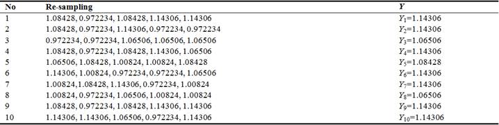
For convenience, suppose BMD population mean is approximated to 1g/cm2 with deviation 0.1g/cm2. Suppose we have simulated BMD sample D = {X1=0.972234, X2=1.06506, X3=1.08428, X4=1.00824, X5=1.14306} of size n=5 which conforms normal distribution with mean 1 and variance 0.12. After re-sampling m=10 times without replacement according to bootstrap technique, we have 10 new maximal observations E = {Y1, Y2,…, Y10} where Yi is maximum value of sample {Xi1, Xi2,…, Xi5} be the maximum value at time i. It is easy to recognize that E is simulated pBMD sample. Note that author [2] also used bootstrap method to obtain pBMD data like I do. Table 1 shows these maximum values.
Suppose Yi conforms Gumbel distribution, we need to estimate its mean ![]() and variance
and variance ![]() where
where ![]() is the estimated pBMD. According to equation (4), the parametric estimates
is the estimated pBMD. According to equation (4), the parametric estimates ![]() and
and ![]() must be determined first with regard to equation (3). We have:
must be determined first with regard to equation (3). We have:

![]()
![]()
Finally, the estimated pBMD is 1.12158 with deviation ![]() . Moreover, the lower-tail percentile point denoted Y0 at significant level 0.025 is:
. Moreover, the lower-tail percentile point denoted Y0 at significant level 0.025 is:
![]()
The upper-tail percentile point denoted ![]() at significant level 0.025 is:
at significant level 0.025 is:
![]()
According to equation (1), given estimates ![]() and
and ![]() , Gumbel density function g(Y) is:
, Gumbel density function g(Y) is:
![]()
Figure 1 shows the graph of such Gumbel density function g(Y) as follows:
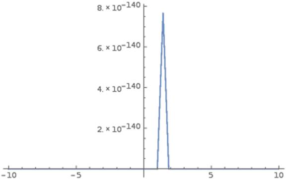
Figure 1. Graph of Gumbel density function.
As seen in figure 1, pBMD data concentrates highly on the peak of density function g(Y) at its mean µ = 1.12158. Although g(Y) is asymmetric, the lower-tail and upper-tail percentile points (1.11979 and 1.12454) at significant level 0.025 are very close to the peak. In other words, 95% confident interval containing the mean µ = 1.12158 is very narrow (0.00475 = 1.12454 – 1.11979), which indicates that such mean is the most likely pBMD.
Following is code snip for pBMD estimation mentioned above, written by Wolfram language built in Mathematica software [7].
m=5;
n=10;
significant=0.025;
(* Simulated sample D with mean 1 and deviation 0.1 *)
x=RandomVariate[NormalDistribution[1,0.1],m]
(* Producing maximal observations E by bootstrap technique *)
yy=Table[RandomChoice[x,m],{i,n}]
y=Map[Max,yy]
(* Estimating parameters such as alpha and beta *)
ymean=Mean[y]
beta=Sqrt[6]/((n-1)Pi)(Sum[(y[[i]])^2,{i,n}]-n*(ymean^2))
alpha=ymean-EulerGamma*beta
(* Estimating mean and variance *)
mu=alpha+EulerGamma*beta
var=beta*Pi/Sqrt[6]
Sqrt[var]
(* Percentile points at significant level 0.025 *)
lowerpercentile=alpha-beta*Log[-Log[significant]]
upperpercentile=alpha-beta*Log[-Log[1-significant]]
g[z_]:=1/beta*Exp[-(z-alpha)/beta]*Exp[-Exp[-(z-alpha)/beta]]
g[z]
(* Plotting the Gumbel density function *)
Image[Plot[g[z],{z,-10,10}]]
4. Conclusion
The ideology of this research is to apply maximum Gumbel distribution into estimating pBMD and its variance by moment technique, instead of using normal approximation to maximal values. This is my main contribution in the area of pBMD estimation. So Gumbel distribution ensures accuracy of estimation and this is the strong point of my method. The drawback is the complexity of estimation when it is required a lot of calculus and arithmetic operations. In the future, I will research how to make approximation of Gumbel distribution so that the derived distribution is simpler than Gumbel distribution.
Acknowledgement
This research is the place to acknowledge Doctor Ho-Pham, Lan T. – Pham Ngoc Thach University of Medicine, Ho Chi Minh city, Vietnam who produces an excellent research [1] from which my research is inspired. Moreover she gave me valuable comments and advices that help me to improve this research.
References


