| 1. | ||
| 2. | ||
| 3. | ||
| 4. | ||
| 5. | ||
New Potential of the
Positron-Emission Tomography
Andrey N. Volobuev1, Eugene S. Petrov2, Peter I. Romanchuk1,
Paul K. Kuznetsov3
1Department of Physics, Samara State Medical University, Samara, Russia
2Department of Operative Surgery, Samara State Medical University, Samara, Russia
3Department of Electric-Drive, Samara State Technical University, Samara, Russia
Email address
 (A. N. Volobuev)
 Citation
Andrey N. Volobuev, Eugene S. Petrov, Peter I. Romanchuk, Paul K. Kuznetsov. New Potential of the Positron-Emission Tomography. International Journal of Modern Physics and Application. Vol. 3, No. 2, 2016, pp. 39-44.
Abstract
On the basis of the reason analysis of the photon angular distribution formed at the electron and positrons annihilation the new potential of the positron-emission tomography for detection of tissue biophysical mechanical parameters is investigated. It is shown that photon angular distribution at electron-positron annihilation is consequence of Doppler’s effect in the reference frame of the electron and positron mass center. In the reference frame bound with electron the photon angular distribution is absent. But it is replaced by the Doppler’s shift of photon frequencies. The estimation of the offered method sensitivity for a finding of tissue parameters is carried out.
Keywords
Annihilation, Electron, Positron, Photon, Doppler’s Effect, Angular Photon Distribution, Positron-Emission Tomography (PET)
1. Introduction
Positron-emission tomograph (PET) is the advanced diagnostic device used for search tumors and its metastases at the earliest stages of their occurrence. However in our opinion of a positron-emission tomography potential are not exhausted yet. The purpose of present paper is to show as with help PET it is possible to find density of a tissue.
The analysis of angular distribution of flying out photons by energy ![]() (
(![]() - Planck's constant,
- Planck's constant, ![]() - photon frequency) at annihilation of a positron
- photon frequency) at annihilation of a positron ![]() and electron
and electron ![]() has great importance for high-grade use of the PET. Unfortunately the mechanism of annihilative process
has great importance for high-grade use of the PET. Unfortunately the mechanism of annihilative process ![]() of the electron and positron is unknown. P. Dirac has been offered model of this process. According to Dirac [1, 2] the annihilation it is possible to present as transformation of the electron from a state with positive energy to the state with negative energy. According to the Dirac’s theory vacuum holes the positron it is the hole in the field of vacuum. Interaction of the electron and positron i.e. them annihilation is a filling vacuum hole by the electron. Thus energy as two quantums of electromagnetic radiation is allocated.
of the electron and positron is unknown. P. Dirac has been offered model of this process. According to Dirac [1, 2] the annihilation it is possible to present as transformation of the electron from a state with positive energy to the state with negative energy. According to the Dirac’s theory vacuum holes the positron it is the hole in the field of vacuum. Interaction of the electron and positron i.e. them annihilation is a filling vacuum hole by the electron. Thus energy as two quantums of electromagnetic radiation is allocated.
2. Angular and Power Distributions of Annihilative Radiations
Quantum-electrodynamical calculations of the annihilative process have been carried out enough for a long time. They were repeatedly checked and rechecked, including authors of the article. As a result of these calculations two formulas for the differential effective section of electromagnetic radiation quantums scattering in a solid angle ![]() have been found.
have been found.
The first formula on time has been found by Heitler [3]. This formula looks like:
. (1)
(1)
The formula is written in designations [4] where there is its detailed deduction. The so-called rational system of units which speed of light and Planck's constant are equal to unit ![]() is used. In this system of the units the energy, impulse and mass have the identical dimension.
is used. In this system of the units the energy, impulse and mass have the identical dimension.
In the formula (1) ![]() there is electron charge (or positron with an opposite sign),
there is electron charge (or positron with an opposite sign), ![]() - the photon energy,
- the photon energy, ![]() - the electron impulse,
- the electron impulse, ![]() - the angle between impulses of the electron and one of the radiated photons. The formula (1) is found under condition of summation on all directions of photons polarization.
- the angle between impulses of the electron and one of the radiated photons. The formula (1) is found under condition of summation on all directions of photons polarization.
At the deduction (1) the reference frame connected to the center of mass interacting the electron and positron is used which the impulses of electron and positron are equal on the module and are opposite on the direction ![]() . Impulses of photons also are equal on the module and opposite on the direction
. Impulses of photons also are equal on the module and opposite on the direction ![]() [3, 4]. We shall note that in this reference frame the condition of both photons supervision are identical.
[3, 4]. We shall note that in this reference frame the condition of both photons supervision are identical.
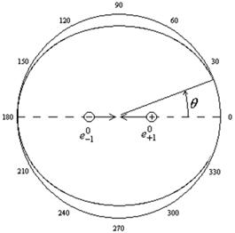
Figure 1. Angular distribution of annihilative radiations.
In fig. 1 the distribution ![]() plotted according to the formula (1) is shown. This distribution is plotted for the ratio
plotted according to the formula (1) is shown. This distribution is plotted for the ratio  . Factor before brackets in (1) is accepted equal to unit. The graph in fig. 1 has illustrative character since actually as it will be shown below
  where
where ![]() there is fine-structure constant [5]. In this case the distribution
there is fine-structure constant [5]. In this case the distribution ![]() there is practically spherical symmetric.
there is practically spherical symmetric.
The second formula which represents frequency or power distribution of the radiated quantums has been offered a little later by Feynman [6]:
![]() (2)
(2)
The formula (2) is written down in designations [6]. As well as in the previous variant (1) the rational system of units is used.
In the formula (2) ![]() and
and ![]() there are unit vectors of photons polarization radiated at annihilation,
there are unit vectors of photons polarization radiated at annihilation, ![]() and
and ![]() - the frequencies of the radiated photons,
- the frequencies of the radiated photons, ![]() - the mass of electron (or positron),
- the mass of electron (or positron), ![]() - the module of the positron impulse,
- the module of the positron impulse, ![]() - its energy.
- its energy.
The formula (2) is similar to Klein – Nishina’s formula for Compton’s effect [6,7]. The main difference there are before the third and fourth addends in the square brackets the signs changed on opposite.
The major distinctive condition of the formula (2) deduction is use of other reference frame in comparison with the formula (1) deduction. The formula (2) was deduced in the reference frame in which electron is at rest, and positron moves.
This reference frame as a whole is equivalent to the reference frame coupled with PET. Therefore we shall name this reference frame as laboratory. The electrons in the substance researched in PET basically are in the bound state. Positrons there are result a ![]() - positron radioactive decay of the shortly-lived radiopharmaceutical isotopes, for example
- positron radioactive decay of the shortly-lived radiopharmaceutical isotopes, for example ![]() . Therefore electrons in laboratory reference frame it is possible to assume motionless (if to exclude chaotic thermal movement of molecules).
. Therefore electrons in laboratory reference frame it is possible to assume motionless (if to exclude chaotic thermal movement of molecules).
Both formulas (1) and (2) were deduced with the help of Feynman standard diagram technique and diagrams of second order of the perturbations theory. However results of the deductions essentially differ.
First, the formula (1) assumes rather complex angular distribution of intensity I of annihilative radiation, since ![]() where
where ![]() there is energy flux of radiation through the area
there is energy flux of radiation through the area ![]() , intensity
, intensity ![]() . And this distribution is connected only to the electron (positron) impulse. The angle
. And this distribution is connected only to the electron (positron) impulse. The angle ![]() is present only at the complex with impulse
is present only at the complex with impulse ![]() . In the formula (2) the distinct form photons angular distribution in the obvious kind is absent.
. In the formula (2) the distinct form photons angular distribution in the obvious kind is absent.
Second, the formula (2) assumes the opportunity of photons various energy at annihilation that is forbidden by the formula (1) deduction owing to ![]() .
.
Therefore, first of all, there is a question what nature of angular distribution of the annihilative radiation intensity in (1)? Whether this distribution with annihilative process i.e. transformation "substance – energy" is connected or that is defined by other effects? Whether the given angular distribution of photons will be kept at transition to other reference frame coupled, for example, to the PET?
3. The Reasons of Angular and Power Distribution of the Annihilative Radiations
For research of the angular dependence reason of differential effective section (1) we shall consider intermediate expression of the deduction which is not summarized yet on directions of the photons polarization [4]:
 ,(3)
,(3)
where ![]() and
and ![]() there are impulses of photons. Variables in square brackets: an impulse of electron, impulses of photons, unit vectors of photons polarization are written down as 4-vectors.
there are impulses of photons. Variables in square brackets: an impulse of electron, impulses of photons, unit vectors of photons polarization are written down as 4-vectors.
The formula (3) is simple for transforming to the kind:
 . (4)
. (4)
Let's transit in (4) to spatial vectors using a rule ![]() where a and b there are three-dimensional vectors,
where a and b there are three-dimensional vectors, ![]() and
and ![]() - in our case power components of 4-vectors.
- in our case power components of 4-vectors.
Transiting to three-dimensional vectors, and also taking into account absence power components at polarizing 4-vectors ![]() the expression (4) it is possible to present as:
the expression (4) it is possible to present as:
 . (5)
. (5)
At deduction (5) the condition of photons flying in strict opposite directions ![]() also is used.
also is used.
Taking into account ![]() , and also according to the energy conservation law
, and also according to the energy conservation law ![]() (for clearly evident it is entered inside brackets the speed of light
(for clearly evident it is entered inside brackets the speed of light ![]() ) in the formula (5) we shall replace
) in the formula (5) we shall replace  , where
 ![]() - speed of electron. In result we shall receive:
- speed of electron. In result we shall receive:
 . (6)
. (6)
Let's transit in (6) to the laboratory reference frame bound with electron. In this case ![]() , and
, and ![]() it is possible to examine as speed of a positron movement. The same there concerns and to value
it is possible to examine as speed of a positron movement. The same there concerns and to value ![]() in factor before brackets (p – positron impulse). In the given reference frame the formula (6) becomes simpler:
in factor before brackets (p – positron impulse). In the given reference frame the formula (6) becomes simpler:
 .(7)
.(7)
We research an auxiliary task.
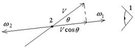
Figure 2. Supervision of the photons which was emitted by the moving particle.
The observer 1 who are taking place in "motionless" (connected with the Earth) reference frame, fig. 2, examines some particle 2 moving with a speed ![]() which in certain moment of time radiated two quantums opposite directed. At
which in certain moment of time radiated two quantums opposite directed. At ![]() the quantum frequency is
the quantum frequency is ![]() . The angle between speed of the particle and direction of one quantum propagation is equal
. The angle between speed of the particle and direction of one quantum propagation is equal ![]() . In the observer direction the particle has a component of speed
. In the observer direction the particle has a component of speed ![]() .
.
Due to Doppler’s effect the quantum moving in the observer direction will have the increased frequency [8]:
 . (8)
. (8)
For the quantum moving in an opposite direction so-called the "red displacement" of frequency will be observed:
 . (9)
. (9)
Using (8) and (9) we shall find size of the complex ![]() which is included into the formula (2):
which is included into the formula (2):
 . (10)
Let's note that distinction in frequencies of quantums in the examined task is determined by distinction in conditions of these quantums supervision: one quantum moves to the observer another leaves from him.
In the formula (7) the considered auxiliary task is actually realized. Thus the moving particle is meant as a positron, and the observer is on "motionless" electron. Therefore substituting (10) in (7) we shall find:
 . (11)
Let's note that at use of the formula (10) we have actually refused the condition ![]() .
.
If in factor before brackets in the formula (2) to use ![]() the formulas (2) and (11) become identical.
the formulas (2) and (11) become identical.
We shall note one important point arising at transition from the reference frame of the electron and positron mass center to the reference frame bound with electron or laboratory reference frame. If to divide the formula (9) on the formula (8) the result which differs from the result received in monographies, for example, [9,10] turns out.
At division (9) on (8) and accepting ![]() we receive:
we receive:
![]() . (12)
. (12)
In [9,10] the following ratio is offered:
![]() . (13)
. (13)
Taking into account ![]() and
and ![]() we find:
we find:
![]() . (14)
. (14)
The formula (14) differs from the formula (12) a little. It is connected by that the formula (14) is received within the framework of the first approximation of the perturbation theory. Therefore it is essentially inexact. The formula (12) follows from exact formulas of Doppler’s effect. Thus remaining only within the framework of the first approximation of the perturbation theory it is impossible to establish equivalence of formulas (1) and (2).
In summary we shall summarize the formula (11) on photons polarization. Coming back to polarizing 4-vectors with the account ![]() also using
also using ![]() [4], we shall find:
[4], we shall find:
 . (15)
The module used owing to standard use of the module of a compound matrix element at the finding of the process differential effective section [3].
4. Application of the Annihilative Radiations in a Positron-Emission Tomograph
Taking into account that in a positron-emission tomography the positrons speed is insignificant, and also taking into account (8) and (9) it is possible to write down:
 . (16)
Substituting (16) in (15), we shall find:
 , (17)
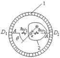
Figure 3. The basic scheme of photons registration in the positron-emission tomography.
Let's find the frequencies difference of radiated photons, i.e. size ![]() , using formulas (8) and (9):
, using formulas (8) and (9):
 . (18)
On fig. 3 the basic scheme of photons registration in the positron-emission tomography [11] is shown.
If the angle ![]() , i.e. a positron moves on the line connecting detectors
, i.e. a positron moves on the line connecting detectors ![]() - radiation
- radiation ![]() and
and ![]() , the difference of the photons frequencies
, the difference of the photons frequencies ![]() will be greatest and the formula (18) will be transformed to the kind:
will be greatest and the formula (18) will be transformed to the kind:
 . (19)
Taking into account ![]() , we shall find:
, we shall find:
![]() . (20)
. (20)
The size ![]() can be found from the approached equality
can be found from the approached equality ![]() . In this case:
. In this case:
![]() , (21)
, (21)
where ![]() there is Compton’s length of an electron wave [12].
there is Compton’s length of an electron wave [12].
Let's estimate the size ![]() . The positron at disintegration used in PET a radiopharmaceutical element takes off with very big velocity close by light speed. But two-photon annihilation it is possible only at small velocity of particles by means of positronium formation [5]. At the big energy of the positron there originate mesons or hadrons. Therefore, for occurrence two-photon annihilation the positron should be slowed down very much. The positronium energy is equal
. The positron at disintegration used in PET a radiopharmaceutical element takes off with very big velocity close by light speed. But two-photon annihilation it is possible only at small velocity of particles by means of positronium formation [5]. At the big energy of the positron there originate mesons or hadrons. Therefore, for occurrence two-photon annihilation the positron should be slowed down very much. The positronium energy is equal ![]() . Believing the positron energy
. Believing the positron energy ![]() in electron electric field to equal half of positronium energy we find the positron impulse from the expression
in electron electric field to equal half of positronium energy we find the positron impulse from the expression ![]() . As positron impulse is small
. As positron impulse is small ![]() the positron velocity is equal
the positron velocity is equal ![]() . Using (21) we shall find
. Using (21) we shall find ![]() . The found difference of frequencies is equivalent
. The found difference of frequencies is equivalent ![]() . If to use energy of an annihilative photon
. If to use energy of an annihilative photon ![]() the received difference of frequencies makes 0.73 %. The given size completely is acceptable to measurement by modern detectors of
the received difference of frequencies makes 0.73 %. The given size completely is acceptable to measurement by modern detectors of ![]() -radiation. Earlier at the estimation of the real form of annihilative radiation distribution, fig. 1, the ratio has been used. Really from the formula
-radiation. Earlier at the estimation of the real form of annihilative radiation distribution, fig. 1, the ratio has been used. Really from the formula ![]() follows
follows  .
.![]()
The researched object 2 is placed in the ring of detectors 1. At the annihilation of a positron and electron, taking place in a point a, the two quantums energies ![]() and
and ![]() in opposite directions radiated (Planck's constant
in opposite directions radiated (Planck's constant ![]() used for clearing). If the quantums flying on line A-A, are registered by detectors
used for clearing). If the quantums flying on line A-A, are registered by detectors ![]() and
and ![]() simultaneously the point of quantums emission is in the middle between detectors
simultaneously the point of quantums emission is in the middle between detectors ![]() and
and ![]() . Detectors in a ring 1 from the point of Doppler’s effect view in the reference frame bound with electrons play a role of motionless observers.
. Detectors in a ring 1 from the point of Doppler’s effect view in the reference frame bound with electrons play a role of motionless observers.
By number of the quantums which are radiated in different directions process is spherical symmetric. Therefore the density of detectors in a ring 1 should be uniform. However the quantum frequencies and consequently also their energy depending on a direction on the detector (observer) due to the Doppler’s effect can be differ on size ![]() .
.
Measuring the frequencies or energies difference of the quantums which radiated opposite directions also using the maximal value of this difference during measurement ![]() it is possible to find the speeds of positrons movement under the formula (21).
it is possible to find the speeds of positrons movement under the formula (21).
The positron velocity depends on mechanical parameters of a tissue through which it moves: density, viscosity, etc. Therefore estimating the positron velocity it is possible to receive the information on mechanical parameters of the tissue in tumor. This additional information can be received during diagnostics of an organism with the help of the positron-emission tomograph.
5. Conclusion
By results of the carried out analysis we can draw the following conclusions.
Formulas Heitler (1) and Feynman (2) it is adequate in different reference frames describe scattering photons at annihilation of electron and positron.
In the laboratory reference frame bound with electron the angular distribution of number photons is spherical symmetric however due to distinction in conditions of quantums supervision owing to Doppler’s effect there is a distinction in frequencies of the radiated quantums.
At transition in the reference frame bound to the center of mass of electron and positron the distinction in frequencies of the radiated quantums is reduced in angular distribution of annihilative photons intensity which also is consequence of Doppler’s effect.
Investigating the angular distribution of electromagnetic radiation intensity at annihilation of a positron and electron in the reference frame of their mass center we research not annihilation, and other physical phenomenon – Doppler’s effect which accompanies with annihilative radiation. Hence the first not disappearing amendment of the perturbation theory received on the basis of a holes Dirac’s hypothesis does not result in confirmation or denying of this hypothesis even if experiments confirm angular distribution of the annihilative radiation intensity.
Measuring the frequencies or energies difference of the quantums which have flung out opposite directions it is possible to find the speeds of positrons movement, see formula (21).
Taking into account the size of positron velocity in the pathological tissue through which it moves it is possible to receive the information on mechanical parameters of this tissue.
References


