| 1. | ||
| 2. | ||
| 3. | ||
| 4. | ||
| 5. | ||
| 6. | ||
| 7. | ||
Adaptive Wavelet Image Denoising Based on the Entropy of Homogenus Regions
Abdolreza Dehghani Tafti1, Serajeddin Ebrahimian Hadi Kiashari2
1Department of Electrical Engineering, Islamic Azad University Karaj Branch, Karaj, Iran
2Department of Mechatronics Engineering, K. N. Toosi University of Technology, Tehran, Iran
Email address
 (A. D. Tafti)
  (S. E. H. Kiashari)
 Citation
Abdolreza Dehghani Tafti, Serajeddin Ebrahimian Hadi Kiashari. Adaptive Wavelet Image Denoising Based on the Entropy of Homogenus Regions. International Journal of Electrical and Electronic Science. Vol. 3, No. 4, 2016, pp. 19-25.
Abstract
In this paper, a new method for adaptive wavelet image denoising is proposed. In the proposed method, the noisy image is segmented to the homogenus color-texture regions by JSEG (J-segmentation). Then, the entropy values of regions are calculated and considered as the estimation of noise complexity in each region. According to the segments’ entropy values, the regions are divided in two clusters; one cluster consists of regions with lower entropy than the mean of entropy values and other cluster is regions with the higher entropy values. Different wavelets are selected for denoising of clusters because the performance of a wavelet in image denoising is different in relation to the level of noise. The regions with higher entropy can be denoised by Db4, which is the wavelet that has better performance when noise level is high, and a common wavelet such as Db2 can be used for denoising in lower entropy regions. Finally, the denoised image reconstructed by composition of denoised regions. The simulation results show that the proposed method produces better denoised image than using of one wavelet in an image.
Keywords
Adaptive Image Denoising, Wavelet Denoising, Entropy, JSEG Method
1. Introduction
Denoising images corrupted with noise is an important part in signal and image processing. Image denoising techniques use to eliminate random noise in images while their features such as edges and textures remain unchanged. One of the significant methods for image denoising is wavelet thresholding. Donoho proposed hard and soft thresholding methods for denoising [1]. Critical parameters in perfect wavelet denoising are estimation of noise and threshold value. Many wavelet image denoising methods, which have been introduced such as [2-7], have focused on statistical modeling of wavelet coefficients and optimal thresholding.
In this paper, with respect to the estimation of noise value with entropy value, a new method to obtain denoised image based on using wavelet is proposed in homogenous color-texture images. At first step, the image is divided to color-texture homogenous regions by JSEG. One of the most robust techniques to identify homogenous regions is JSEG [8]. Because of amorphous shape of regions in JSEG method, a rectangular shape can be considered for each region. After that, the entropy of each region is calculated and considered as estimation level of noise. Based on the entropy values, the regions are clustered in two clusters. First cluster consists of regions which their entropies values are higher than mean of all entropies and second cluster consists of other regions. Next, the suitable wavelet can be associated to each cluster. In cluster with high entropy regions, an effective wavelet such as Db4 or Db8 and for low entropy regions, common wavelet such as Db2 can be used effectively in image denoising [9]. After denoising the regions with associated wavelet, the final denoised image is reconstructed by separate denoised regions. If a rectangular shape is considered for each region, there are several overlapped pixels between regions. In this situation, the mean value of overlapped pixels can be considered to obtain final value for these pixels. The quality of denoised image improves significantly by using different wavelet adaptively.
This paper is organized as follows: In Section 2 the wavelet image denoising is discussed. In Section 3 and 4, JSEG method and image entropy will be described briefly, respectively. In Section 5 the new method is proposed, and finally simulation results and conclusions have been discussed in Section 6 and 7.
2. The Wavelet Image Denoising
Generally wavelet image denoising consists of three steps. A linear wavelet transform, a nonlinear thresholding with one of two functions that summarized at hard and soft thresholding, and inverse wavelet transform.
In the first step, wavelet transform is applied by a chosen wavelet. Then, the noise can be estimated in wavelet domain by following equation [1]:
![]() ,
,![]() (1)
(1)
where L is the number of wavelet decomposition and ![]() stands for median function. There are many ways to find threshold number [1], [3], [4]. As a common method, it is given by
stands for median function. There are many ways to find threshold number [1], [3], [4]. As a common method, it is given by
![]() (2)
(2)
where the ‘σ’ is estimated noise which can be obtained by (1). According to the equation (2) it can be seen that the threshold number is related to estimated noise and image size (![]() ). Then, wavelet coefficients can be thresholded by one of two functions, hard threshold and soft threshold. In the hard thresholding, function keeps the input if it is larger than threshold and otherwise set input to zero. The soft thresholding function shrinks coefficients that under threshold till zero. If
). Then, wavelet coefficients can be thresholded by one of two functions, hard threshold and soft threshold. In the hard thresholding, function keeps the input if it is larger than threshold and otherwise set input to zero. The soft thresholding function shrinks coefficients that under threshold till zero. If ![]() ,
, ![]() denote the input and output then follow equations describe them clearly.
denote the input and output then follow equations describe them clearly.
Hard threshold: 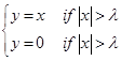 (3)
(3)
Soft threshold: ![]() (4)
(4)
The hard and soft thresholding functions are shown in Fig. 1. Clearly, the choice of the threshold plays an important role in image denoising. After thresholding, the inverse wavelet transform can be applied to obtain the denoised image.
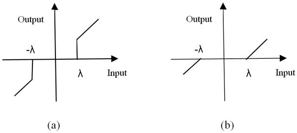
Fig. 1. Thresholding functions; (a) the hard threshold function. (b) the soft threshold function.
3. The Jseg Method for Image Segmentation
One of the most effective algorithms for unsupervised segmentation of color-texture regions in image and video is JSEG (J-segmentation) [8]. This algorithm segments image and video to homogenous color-texture regions. It has two steps, color quantization and spatial segmentation which is shown in Fig. 2. In color quantization step, colors in image are quantized into several classes, this quantization can separate regions in image and corresponding color class labels, which is replaced the original pixel values, create a class map. In second step, spatial segmentation will be done according to the class map. By defining J value for local windows (scales) in the class-map, the J-image is obtained. To clarify, let ![]() be the set of all
be the set of all ![]() data points in a class-map. If
data points in a class-map. If ![]() represents the image pixel position (i.e.,
represents the image pixel position (i.e.,![]() ) then the mean
) then the mean ![]() can be obtained by:
can be obtained by:
![]() (5)
(5)
Now, assume ![]() is classified into
is classified into ![]() classes,
classes, ![]() ,
, ![]() =
= ![]() , …,
, …, ![]() . Let
. Let ![]() be the mean of the
be the mean of the ![]() data points of class
data points of class ![]()
 (6)
(6)
let
![]() (7)
(7)
and
![]() (8)
(8)
SW is the total variance of points which are belonging to the same class. The J is defined as
![]() (9)
(9)
The ![]() value can be calculated for each pixel in a small window centered at the pixel. Also, the size of local window determines the size of image regions that can be detected which is shown in Table 1 [8]. The high and low values of the J-image represent the region boundaries and region interior, respectively. Therefore, a region growing method to segment the image can be used according to the J-image [9].
value can be calculated for each pixel in a small window centered at the pixel. Also, the size of local window determines the size of image regions that can be detected which is shown in Table 1 [8]. The high and low values of the J-image represent the region boundaries and region interior, respectively. Therefore, a region growing method to segment the image can be used according to the J-image [9].
Table. 1. Window sizes at different scales in the JSEG method.
| scale | Window (pixels) | Sampling (1/pixels) | Region size (pixels) | Min. seed (pixels) |
| 1 | 9×9 | 1/(1×1) | 64×64 | 32 |
| 2 | 17×17 | 1/(2×2) | 128×128 | 128 |
| 3 | 33×33 | 1/(4×4) | 256×256 | 512 |
| 4 | 65×65 | 1/(8×8) | 512×512 | 2048 |
To clarify, the result of JSEG method with different scales in segmentation of a satellite image (Azadi Square in Iran) are shown in Fig. 3.
Fig. 2. Schematic of the JSEG algorithm for color image segmentation [8].
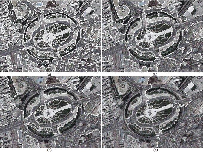
Fig. 3. The segmented Image with JSEG method; (a) Scale 1. (b) Scale 2. (c) Scale 3. (d) Scale 4.
It can be seen that, at scale 1 and 2 the number of regions is too high and it makes a problem with high computation burden. Also, when the scale is 4, the number of regions becomes low and precision is missed. The scale 3 can be selected as a good scale for segmentation.
4. The Image Entropy
Entropy, which is defined by Shannon, can be considered as a measure of uncertainty about information [10]. Shannon’s work is based on the concept of the information gain from an event is inversely relate to its probability of occurrence [10]. Several authors have used Shannon concepts for image processing problems [11-13]. The entropy of a gray scale image from Shannon’s concept is given by [10]:
![]() (10)
(10)
where ![]() represents the number of times that the
represents the number of times that the ![]() th gray level appears in an L-gray-level image and
th gray level appears in an L-gray-level image and ![]() is the total number of pixels in the image. After the segmentation of image with JSEG method, the effect of noise in regions can be analyzed based on the entropy value for each region since entropy can explain the complexity of image [11-13]. In each region which noise has serious effect, entropy value will be higher and in regions with low effect of noise the entropy value will be lower. In Fig. 4, the frequency distribution graph for entropies of segments of Fig. 3 (c) is shown.
is the total number of pixels in the image. After the segmentation of image with JSEG method, the effect of noise in regions can be analyzed based on the entropy value for each region since entropy can explain the complexity of image [11-13]. In each region which noise has serious effect, entropy value will be higher and in regions with low effect of noise the entropy value will be lower. In Fig. 4, the frequency distribution graph for entropies of segments of Fig. 3 (c) is shown.
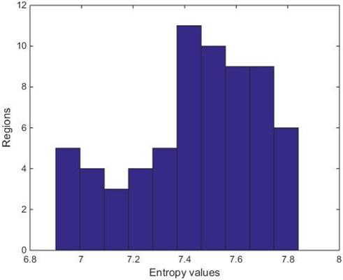
Fig. 4. The frequency distribution graph for entropies of Regions.
As it can be seen in Fig. 4, regions can be divided into two clusters. One cluster consists of the regions that their entropies are lower than the average of entropies and other cluster is regions with higher entropy than the average. As a result of the relation between entropy and uncertainty, the regions with high entropy can be considered as regions with high value of noise, and regions with low value of entropy as regions with low value of noise.
5. Proposed Method
After applying JSEG method on noisy image, the entropy value of each region is calculated, then based on the frequency distribution graph for entropies of segments, regions are divided in two main parts. Regions with high entropy value are taken as high noise regions and regions with low entropy are taken as medium noised regions. After clustering, the wavelet image denoising on each cluster with respect of the entropy value is applied. For regions with high noise an effective wavelet such as Db4 or Db8 can be selected and for low noise regions a common wavelet such as Haar or Db2 may be chosen [14]. After choosing the wavelet adaptively, wavelet image denoising method on each region is applied.
For simplicity, each segment can be considered as a rectangle shape and mentioned procedure is applying to obtain denoised image. The average values for overlapped pixels can be used in reconstructing denoised image.
Simulation results demonstrate that choosing different wavelets for denoising in an image according to the estimation of noise in each region, which can be represented by entropy value of region, can provide better denoised image in compare with denosing by one wavelet.
6. Simulation Results
The performance of proposed method in image denosing can be evaluated by peak signal to noise ratio (PSNR) which is given as,
![]() (11)
(11)
where ![]() is the original image,
is the original image, ![]() is the denoised image and
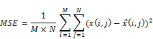
is the denoised image and ![]() represents the size of the image. The PSNR is used to compare the original image and the denoised image. There is an inverse relationship between PSNR and MSE, which is the mean squared error between the original image and the denoised image. Therefore, a higher PSNR value indicates the higher quality of the denoised image. To evaluate performance of proposed method, it is applied to test images which are a satellite image, a medical image, a PCB image, and a nature image which are shown in Fig. 5, Fig. 6, Fig. 7 and Fig. 8, respectively. Test images are contaminated with Gaussian white noise at different standard deviations. The denoised images are obtained by Db2 wavelet, Db4 wavelet and the proposed method, which is used Dd2 and Dd4 adaptively in different regions of image based on the proposed algorithm. The PSNR values for denoised images at different noise covariance for all methods are calculated and reported in Tables.
represents the size of the image. The PSNR is used to compare the original image and the denoised image. There is an inverse relationship between PSNR and MSE, which is the mean squared error between the original image and the denoised image. Therefore, a higher PSNR value indicates the higher quality of the denoised image. To evaluate performance of proposed method, it is applied to test images which are a satellite image, a medical image, a PCB image, and a nature image which are shown in Fig. 5, Fig. 6, Fig. 7 and Fig. 8, respectively. Test images are contaminated with Gaussian white noise at different standard deviations. The denoised images are obtained by Db2 wavelet, Db4 wavelet and the proposed method, which is used Dd2 and Dd4 adaptively in different regions of image based on the proposed algorithm. The PSNR values for denoised images at different noise covariance for all methods are calculated and reported in Tables.
The data in Tables show that the proposed method has the highest PSNR value for each image at each level of noise. Therefore, its performance is better than the classical wavelet denoising method that a constant wavelet is used for image denoising [14].
7. Conclusion
The wavelet image denoising is discussed in this paper and an adaptive method for this purpose is introduced. Since the quality of denoised image depend on the used wavelet, choosing appropriate wavelet is an important issue. Some wavelet such as Db4 or Db8 provide better results when the noise level is high and other wavelet like Haar or Db2 has better performance with low level noise. A new method with the ability of choosing different wavelets in an image can increase the quality of denoised image. Therefore, in the proposed method, the image is segmented to the homogenous segments using JSEG. The entropy of each region is calculated and considered as the estimation of noise level. Then, the entropies of regions are clustered and appropriate wavelet are associated to the each cluster. Finally, the denoised regions are used to obtain the final denoised image. To demonstrate the performance of the proposed method several simulations have been done by MATLAB wavelet toolbox and image processing toolbox. The results show that the priority of proposed method to the wavelet image denoising method. Also, since the segmentation of signal is considered in dynamic sensing, the proposed method should be used for sensor application which can be studied in future researches.
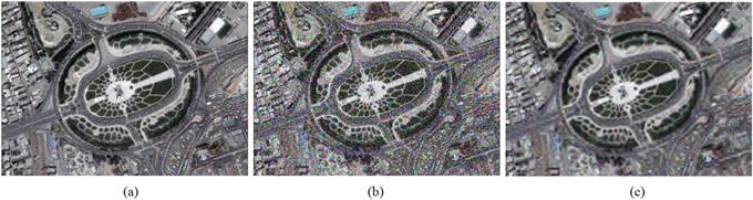
Fig. 5. A satellite image; (a) Original image. (b) Noisy image. (c) Denoised image.
Table 2. The PSNR values of denoised satellite image.
| Noise covariance | PSNR value | ||
| wavelet | Proposed method | ||
| Db2 | Db4 | ||
| 0.01 | 68.8873 | 69.2103 | 70.5877 |
| 0.05 | 67.6585 | 67.9196 | 68.3773 |
| 0.1 | 66.8250 | 67.0257 | 67.2860 |
| 0.15 | 66.2217 | 66.3841 | 66.5811 |
| 0.2 | 65.7583 | 65.8966 | 66.0660 |
| 0.3 | 65.1264 | 65.2350 | 65.3710 |
| 0.5 | 64.2817 | 64.3717 | 64.4908 |
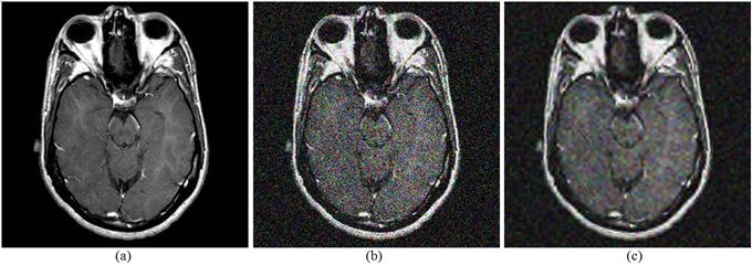
Fig. 6. A MRI image; (a) Original image. (b) Noisy image. (c) Denoised image.
Table 3. The PSNR values of denoised MRI image.
| Noise covariance | PSNR value | ||
| wavelet | Proposed method | ||
| Db2 | Db4 | ||
| 0.01 | 73.1110 | 73.5535 | 74.6099 |
| 0.05 | 68.2550 | 68.4430 | 68.9368 |
| 0.1 | 65.9938 | 66.0963 | 66.3615 |
| 0.15 | 64.6208 | 64.6891 | 64.8319 |
| 0.2 | 63.6291 | 63.6791 | 63.7761 |
| 0.3 | 62.3333 | 62.3638 | 62.4306 |
| 0.5 | 60.8365 | 60.8552 | 60.8983 |
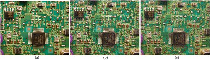
Fig. 7. A PCB image; (a) Original image. (b) Noisy image. (c) Denoised image.
Table 4. The PSNR values of denoised PCB image.
| Noise covariance | PSNR value | ||
| wavelet | Proposed method | ||
| Db2 | Db4 | ||
| 0.01 | 67.1400 | 67.3585 | 69.6036 |
| 0.05 | 65.6743 | 65.7929 | 66.8741 |
| 0.1 | 64.8641 | 64.9800 | 65.5535 |
| 0.15 | 64.3427 | 64.4277 | 64.7677 |
| 0.2 | 63.9183 | 63.9865 | 64.1798 |
| 0.3 | 63.3009 | 63.3661 | 63.4682 |
| 0.5 | 62.5418 | 62.5691 | 62.6717 |
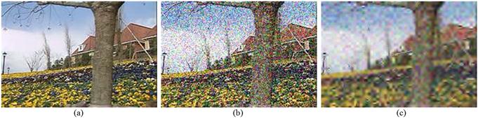
Fig. 8. A natural image; (a) Original image. (b) Noisy image. (c) Denoised image.
Table 5. The PSNR values of denoised natural image.
| Noise covariance | PSNR value | ||
| wavelet | Proposed method | ||
| Db2 | Db4 | ||
| 0.01 | 67.0878 | 67.0864 | 68.1671 |
| 0.05 | 65.9497 | 65.9725 | 66.3131 |
| 0.1 | 65.2096 | 65.2223 | 65.3741 |
| 0.15 | 64.5813 | 64.6115 | 64.7067 |
| 0.2 | 64.1334 | 64.1439 | 64.2387 |
| 0.3 | 63.4788 | 63.4770 | 63.5777 |
| 0.5 | 62.5812 | 62.6113 | 62.6711 |
References


