Modeling of Chlorine Decay Rates in Distribution Systems Based on Initial Chlorine, Reactant Concentrations and Their Distributions
Ababu T. Tiruneh1, Amos O. Fadiran2, Stanley J. Nkambule1,
Lwazi M. Zwane1
1Department of Environmental Health Science, University of Swaziland, Mbabane, Swaziland
2Department of Chemistry, University of Swaziland, Kwaluseni, Swaziland
Email address

(A. T. Tiruneh)

(A. O. Fadiran)

(S. J. Nkambule)

(L. M. Zwane)
Citation
Ababu T. Tiruneh, Amos O. Fadiran, Stanley J. Nkambule, Lwazi M. Zwane. Modeling of Chlorine Decay Rates in Distribution Systems Based on Initial Chlorine, Reactant Concentrations and Their Distributions. American Journal of Science and Technology. Vol. 3, No. 3, 2016, pp. 53-62.
Abstract
A mathematical model for determining the rate of variation of bulk decay rates of chlorine residuals is proposed taking into account factors such as the initial chlorine concentration, the concentrations of reactants and their relative distribution. The theoretical model we built in this research clearly shows that the variation of the bulk decay coefficient with initial chlorine concentrations can be modelled mathematically as a second order reaction which can be easily integrated in modelling programs such as the EPANET. Experiments were carried out for determining the bulk decay rate of chlorine residuals at different initial chlorine doses and the data adequately fit the developed model. We also developed chlorine decay mathematical models for the variation of the rate of reaction of both time-varying as well as time-averaged reaction rates. It is shown that the parameters affecting the variation of reaction rate include: The chlorine concentration and the molar concentration of the low concentration reactants as expressed through the ratio of arithmetic mean to the harmonic mean of the reactant concentrations. For the time-averaged model that can be used in modelling programs based on first order reactions, the time variation of the rate of reaction was additionally influenced by the aggregate (total) reactant concentrations.
Keywords
Chlorine Residual, Bulk Decay Rate, Water Quality, Water Distribution, Reaction Rate, Initial Chlorine Concentration, Variable Rate Chlorine Decay
1. Introduction
Chlorine residual in water distribution systems is among the most important parameters needed for ensuring the standard of potable water supplies [1]. Chlorine dosages in distribution systems are determined primarily by the need to ensure minimum chlorine residual in the distribution system water in order to eliminate microorganisms that are disease causing or that adversely affect the taste and quality of the distributed water as well as the condition of the distribution system. On the other hand, control of excess chlorine doses is required to reduce the extent of formation of disinfection by-products (DBPs) that are known for pausing health related risks in humans [2]. In developing countries, intermittent supplies are common in which some of the water that stays stagnant for longer period of time may be drawn with reduced or no chlorine residual before the fresh supply reaches the consumers [3]. In addition, distribution systems with old ages and unlined iron pipes increase the extent of residual chlorine loss through a combination of losses by microbial growth products and corrosion by-products [4].
Chlorine dosages to water in distribution systems must be optimally adjusted in accordance with the quality of treated water, the rate of decay in the system and the residuals that must be maintained. The optimal solution is essential so that the chlorine residual is not too low running the risk of recontamination of the distribution water or too high which is costly and can generate odour complaints besides having the potential to form disinfection by-products [5].
There are mainly two parallel reactions involved in the decay of chlorine in the distribution system consisting of bulk decay and wall decay. The two processes display different dynamics of chlorine decay and it is difficult to reallocate the portion of decay from the resultant decay within the distribution system corresponding to either of the two processes. Modelling, therefore, requires separate determination of the bulk decay and wall decay parameters [5]. One method by which the wall decay is determined is by subtraction of the bulk decay determined in a laboratory bottle test from the total decay determined from a pilot pipe distribution loop set up [6]. Different pipe materials exhibit different wall decay rate of chlorine [7]. However, chlorine decay coefficients determined from laboratory and pilot tests alone may not be representative of the actual conditions in the distribution system and the model parameters need to be calibrated against actual condition of the distribution system using developed water quality models such as the EPANET [8].
Mathematical modelling of chlorine decay in distribution systems is essential in order to be able to predict chlorine residuals with reasonable accuracy and reduce the cost and time associated with monitoring. In large distribution systems, monitoring of chlorine residuals may be prohibitively expensive [9]. Once the bulk decay and wall decay coefficients are known, the differential equation of chlorine decay with time, expressed in terms of the advective transport and reactive decay, is solved by combining it with conservation of chlorine mass equations established for each node [10].
The most commonly employed model of chlorine residuals in distribution systems is one based on the simple first order decay reaction ([2], [3]). The first-order decay model is a pseudo first order reaction model in which the effect of the reactant with the chlorine compound is not explicitly stated and is, therefore, implicit in the reaction rate constant. This means that when the reactant concentration such as the natural organic matter increases, the reaction rate constant does not stay constant and increases as well. Other models have been developed that take into account the reactant effect [11]. This, as mentioned above, is partly motivated by the fact that the rate of reaction of chlorine is variable, being greater at the beginning of reaction and reducing afterwards whereas the duration of such rate depends, among others, on the initial chlorine concentration [12]. Such difference in rate of reaction may for example be caused by the presence of organic matter which reacts faster with chlorine in the beginning and such reaction being succeeded by the slower reactions involving other chlorine consuming compounds.
There are several reactant based models that are more complex than the simple pseudo first order reaction based model. They all try to take into account the deviation from first order reaction for the decay rate of chlorine when the entire curve of decay is taken into account. One such example of reactant based model is the second order two-reaction model involving fast and slow reactants [13]. Other examples of reactant dependent chlorine decay models that are based on second order models or a combination of first and second order models include the models developed by Clark [14], Jedas-Hecart [15], Ventresque [16], Dharmarajah [17] and Hua et al. [18].
Some authors, however, claimed that the difference in chlorine residual prediction between the more complex models and the ones based on the simple first order reaction is not of much practical significance ([19], [20], [21]).
The fact that the rate of decay of chlorine is variable on a number of factors including, among others, the initial chlorine concentration has been reported by a number of researchers ([22], [18], [20], [7], [12]). Attempts to model the decay rate by empirical relationship taking account of such factors as temperature, initial chlorine concentration, oxidisable organics and inorganics, have been made by several researchers. Hua et al. [18] developed one such integrated model taking account of several factors for the chlorine decay modelling. Hallam et al. [7] also established an inverse relationship between initial chlorine concentration and the reaction rate for the decay of chlorine. However, the inverse relationship as given by Hallam et al. [7] is specific to the test and there is no general model equation or theoretical background given to such variation. It is to be recalled that the inverse relationship has also been observed by several other researchers ([20], [23], [24], [18]).
Other modelling attempts that take into account the effect of initial concentration of chlorine do so by developing parallel models for several assumed initial chlorine doses or establishing ranges of validity. One example of such model is the two-reactant model developed by Fisher et al. [13] in which the two reactant model for chlorine decay is calibrated against maximum and minimum initial chlorine concentrations and the model is expected to fit the data for chlorine dosage ranges in between the maximum and the minimum. However, the use of invariant set of reaction rate parameters for modelling chlorine decay under different initial chlorine concentrations has doubtful outcome given that the rate of reaction is inversely related to the initial chlorine concentration. Similar claims claimed by Kastl et al [25] of model parameters being invariant for initial chlorine concentration ranges between 1 and 4 mg/L has also doubtful universal validity as the invariance may be specific and caused by the fact that the easily reacting organic species in water may not be present in significant concentrations.
Phillip et al. [5] developed a second order time dependent rate of decay model. The model is first order with respect to time dependent chlorine residual and second order with the rate of decay itself. The model uses numerical solution of two differential equations simultaneously, namely, the chlorine decay rate equation and the time dependent rate equations. Euler method was used to solve the equations. The model also uses calibration of the four parameters required by the two differential equations using bulk decay data. Complex evolutionary algorithms were used to find the optimal values of the parameters. Overall the model has no analytical solution and has to use numerical procedure to model the chlorine decay.
2. Materials and Methods
The research work followed a combination of theoretical model development supported by laboratory experiments to verify the model. The theoretical basis for the variation of rate of reaction for the decay of chlorine is formulated by considering two cases. These cases are:
Case I: Chlorine decay modeling based on reaction rate constant that is averaged both over time as well as initial reactant concentration. Such models are common and are expressed by first order reaction with respect to the residual chlorine concentration. The reactant concentration is implicit in the rate.
Case II: Chlorine decay modeling based on time varying but concentration averaged reaction rates. Such models are second order in nature and take account of the effect of the variation of the chlorine and reactant concentrations. The rates are concentration averaged because of the difficulty of deconvoluting the aggregate reaction rates to the individual rates of the different reactant species present.
The experimental part of the research addressed the case of the variation of the time as well as concentration-averaged reaction rates with initial concentration of chlorine as suggested by the developed model equations. Since the effect of reactants is implicit in the model and varies when the water quality conditions of the sample change, the experiment is carried out on a single sample set where the water quality is not expected to change. The experimental procedure as given below was followed.
2.1. Experimental Procedure
The experimental design consisted of collecting a single set of samples from the Matsapha water treatment plant and determining the bulk decay rate coefficients at various different initial concentrations of chlorine. This experiment had the objective of testing the theoretical model that describes the variation of bulk decay coefficient with initial chlorine concentration. The samples collected were treated water samples that passed through the processes of coagulation, flocculation, sedimentation and filtration but that did not pass through the chlorine disinfection system. The single set of samples that are studied are expected to contain homogenous reactant characteristics since the rates determined are the ones based on first order reaction rate models that will obviously change whenever the water quality characteristics change.
The collected samples were immediately brought to the University of Swaziland chemistry laboratory and were tested for chlorine residuals after different known amounts of chlorine were added to various samples tested.
For the determination of chlorine residuals in water samples, the Iodometric titration as outlined in the Standard Methods for the Examination of Water and Wastewater [26] was used. The method is based on the principle that when potassium iodide is added to a sample of water containing residual chlorine at pH of 8 or less, the residual chlorine liberates iodine from the potassium iodide and the liberated iodine is titrated with Sodium thiosulphate (Na2S2O3) titrant.
In order to make the titration stoichiometric, the pH of the sample is reduced to between 3 and 4 by adding acetic acid. The method has expected detection limit of 0.04 mg/L if 0.001 N sodium thiosulphate titrant is used. All chemicals used had reagent grade quality and fresh solutions were prepared every time the experiment was repeated at different time periods.
Depending upon the concentration anticipated, suitable sample volume was taken so that the titrant Sodium thiosulphate (Na2S2O3) volume would not exceed 20 mL and the starch indicator volume also is above 0.2 mL. To the sample volume, 5 mL acetic acid was added followed by 1 g of potassium iodide powder measured on weighing balance. After this, the sample was titrated with Sodium thiosulphate (Na2S2O3) of appropriate normality. For samples with low anticipated chlorine concentrations, the titrant was prepared to be of low normality. The titration was continued until the yellow colour was almost disappearing. Then 1 mL of the starch solution was added until the blue colour disappeared. In order to compensate for method error, blank titration was also performed using distilled-deionized water and that passed through the same procedure as the one used for the actual sample. A minimum of three repetitions were performed for each determination. After titration, the mg/L of chlorine residual present in the sample was determined using the formula:
 (1)
(1)
Where A is the volume of titrant used for the sample, B was the volume of titrant used for blank. N is the normality of the Na2S2O3 titrant.
2.2. Statistical Analysis
After the chlorine residuals were determined for the series of samples to which different known concentrations of chlorine were added, the data were plotted graphically using the log linear plots of concentration versus time using the SPSS statistical package. The SPSS program was also used to carry out regression analysis and determine the parameters for modeling decay of chlorine. In addition, the SPSS statistical package was also used to test for the normality of the residuals after the second order reaction rate model was fitted to the experimentally determined data. The tests used for assessment of normality of residuals were the Q-Q plot and the Shapiro-Wilk test.
2.3. Theoretical Basis for the Time Dependent Rate of Variation of the Reaction Rate with Chlorine and Reactant Concentrations
The following hypotheses are forwarded for the modeling of chlorine residuals in distribution systems based on available data and information for variation of the reaction rate with time
1. For chlorine decay modeling based on time varying but concentration averaged reaction rates, the variation of the rate chlorine decay follows a second order reaction with the rate itself and first order with the residual chlorine concentrations.
2. For the time as well as concentration averaged reaction rate constant of chlorine decay, usually expressed by first order reaction with respect to residual chlorine concentration:

The reaction rate constant K is not constant but varies inversely with initial chlorine residual present and directly with initial concentration of reactants present.
3. For both time varying and time average reaction rates, the time dependent rate of reaction is influenced by the reactant with the lowest molar concentration and this variation is expressed by the ratio of the arithmetic mean to harmonic mean of the reactant concentrations.
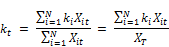
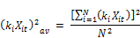
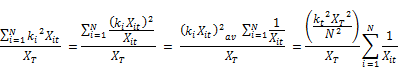
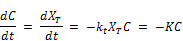
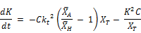
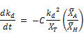
According to Phillip et al. (2009), the time varying – concentration averaged rate of change reaction rate is given by the following equation
 (2)
(2)
Where kt is the concentration weighed reaction rate, Ct is the residual chlorine concentration at time t, Xit is the molar concentration of reactant (i) at time t, XT is the total moles of reactants reacting with chlorine and N is the total number of reactants present in the water.
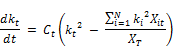
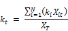
The concentration weighed reaction rate kt is given by:
Where ki is the constant rate of reaction of reactant xi with chlorine and the other variables are described above. From Equation 2 it is apparent that the rate coefficient is variable with respect to time showing linear increase with the concentration of chlorine and being second order with respect to the rate coefficient itself. Other authors ([20], [23], [24], [18]) also observed that the rate constant appears to decrease with increase in the initial concentration of chlorine. Phillip et al. [5] also stated that the rate is negative as the expression in bracket can be shown to be always negative or zero if the rate constants are the same for all the constituents reacting with chlorine. It is also apparent from the equation that the rate variation with time (dkt/dt) is first order with the concentration of chlorine (Ct) and second order with kt. The rate appears to decrease faster for higher concentration of chlorine and is the reason why the apparent overall reaction rate constant is lower for higher concentration of chlorine, a fact observed by several other researchers.
Equation (2) developed by Phillip et al. [5] can be extended, in our opinion, to establish the relationship between the reaction rate variation with chlorine and reactant concentrations as outlined in the hypothesis. It will be shown later in the results section that the experiments performed also confirm more or less the particular case of second order rate relationship between the chlorine decay rate constant and the initial concentration of chlorine.
The analytical expressions for the time varying but concentration averaged rate of reaction (kt) and the time as well as concentration averaged rate of reaction (K) is here by developed on case by case basis. First we consider the expression for the time varying but concentration averaged rate of reaction (kt).
Case I Analytical expression for the time varying concentration weighed rate of reaction
Considering the rate expression proposed by Phillip et al. (2009):
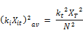
The indeterminate expression in the above equation is the term containing kis because of the difficulty of determining the reaction rate constant for the individual reactants. It is now attempted to get around this problem by reformulating the above equation.
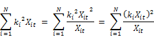
This expression can be expressed as weighted average of the 1/X variable as follows:
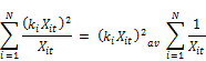
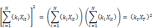
Since:
Therefore,
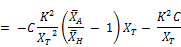
Rearranging further;
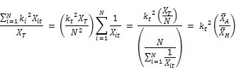
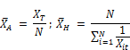
Where XA and XH are the arithmetic and harmonic means of the reactant concentrations respectively. According to the commonly accepted definition of averages, these means are defined as:
Finally the rate expression for the decay of chlorine is given by:
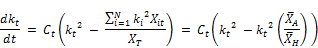
 (3)
(3)
Equation (3) thus expresses the variation of reaction rate in terms of known concentrations, namely the chlorine residual and the arithmetic and harmonic means of the reactant concentrations. This equation can be used to model the variation of reaction rate for the decay of chlorine with time given that these concentrations are known in advance. The individual reaction rates vanish from the equation and are replaced by the ratios of the two averages of reactant concentrations, namely arithmetic and harmonic means.
Since the arithmetic mean XA is always greater than the harmonic mean XH, the expression in the bracket of Equation (3) above is always greater than or equal to zero, i.e.,:

This means that the reaction rate has a negative rate and decreases with time. It is also clear from Equation (3) that the rate of reaction retains the second order rate variation as well as the fact that the rate decreases faster with increase in the chlorine dose. In terms of the overall time-averaged reaction rate, when the initial concentration of chlorine is high, the average slope of the chlorine decay curve become flatter. This is in line with what is commonly reported in the literature about the inverse relationship between reaction rate and initial chlorine concentration.
What is also apparent in Equation (3) is the influence of the concentration of the slowest reacting substance as expressed by the ratio of arithmetic to harmonic means of the reactant concentrations. Accordingly, the reaction rate falls faster with the presence of low concentration reactants that depress the harmonic mean further. In terms, of first order rate modelling, water that is dominated by low concentration of chlorine consuming substances tends to have flatter slope of the chlorine decay curve than otherwise. If the reactants concentrations are comparable, the arithmetic mean and harmonic means approach each other. In this case, the reaction rate remains constant as the expression in bracket in Equation (3) tends to zero. This is typically a situation where the first order kinetic modelling is applicable as the rate of reaction stays constant.
Case II: Analytical expression for the time and concentration averaged rate of reaction
There are two alternatives for deriving the rate expression for the time and concentration- averaged reaction rate for the decay of chlorine applicable for first order modelling. The first alternative is to use the series of steps similar to the steps used in developing the equation for the time varying rate presented above. The second alternative is to use the results of Equation (3) and derive the rate expression from this equation. Both alternatives yield the same result. The second alternative is presented in this paper below
The time and concentration-averaged reaction rate K is expressed in terms of the time varying and concentration-averaged rate from the following:
So that;

Differentiating the rate expression with time;
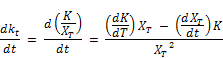
Rearranging the above equation, the rate variation for K becomes;
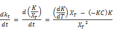
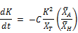
Substituting the expression of Equation for dkt/dt:
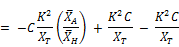
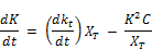
Finally;
 (4)
(4)
Equation (4) is the time dependent rate expression for the concentration as well time-averaged reaction rate. The influence of chlorine concentration and the ratio of arithmetic mean to harmonic mean of the concentration of reactants is also retained in this equation. The influences of these variables are the same as those described for the conditions of Case I above.
The additional factor appearing in Equation (4) is the influence of reactant concentrations as expressed by the variable XT which is the total mole of reactants. When the reactant concentrations are high, the reaction rate falls slower and the slope of the overall decay curve thus becomes steeper. On the contrary, if the concentration of reactants is low, the rate of reaction falls faster and the overall slop of decay becomes flatter.
In other words, the overall time and concentration averaged rate of chlorine decay increases when:
i. The initial reactant concentration increases and
ii. The initial chlorine concentration decreases
The experiments performed addressed case II (ii), i.e., the effect of initial concentration of chlorine on the overall reaction rate. This case is preferred because most chlorine residual modeling programs such as the EPANET are based on first order reaction rate modeling and because of the fact that for the treated water in the Matsapha water treatment plant, the variation of reactant concentration may not be high. However, this condition will be explored by further research in future.
The theoretical basis of the experiment performed for investigating the effect of initial concentration of chlorine is further developed below.
2.4. Second Order Model Formula for Modeling Reaction Rate Variation with Respect to Initial Chlorine Concentration
The rate of decay of chlorine is modeled as usual following a first order reaction as follows:

Where C is the concentration at t, t is the time usually converted to unit of days and kd is the rate of reaction for the bulk decay of chlorine in water inside the distribution system. The symbolic change in the rate of reaction from K to kd is to be noted for the purpose of accommodating additional reaction rate constant for the second order modeling of initial chlorine concentrations.
Referring to Equation (4) again:
In terms of the substituted symbol for K = kd:
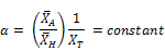
If the reactant types and their concentration remain the same as is the case in the experiment performed in this research;

Where;
If the initial chlorine concentration is made to vary, then the rate of reaction is now a function of two variables namely time and initial chlorine concentration.

The above expression can also be written as;

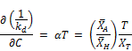
Differentiating the above equation with respect to the chlorine concentration again
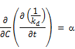
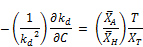
Reversing the order of the partial differentiation above;
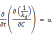
Integrating to the entire time range T where the overall decay rate kd covers all the data and the concentration approaches zero (i.e., C = 0 at t = T)
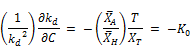
Where the initial concentration based decay rate K0 is given by:

The expression above now becomes:
 (5)
(5)
Where C is the initial concentration of chlorine, K0 the rate constant for concentration based reaction rate.
Integrating between the initial rate at C0 = 0 and at any given initial concentration Co gives;
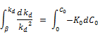
Where b is the initial reaction rate constant when the initial concentration of chlorine approaches zero.
After integration the expression becomes;
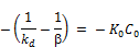
Finally:
 (6)
(6)
The regression based modeling is carried out by linear regression of (1/kd) against the initial concentration for a number of chlorine decay tests carried out at different initial concentrations of chlorine. The regression parameters b and K0 are determined from this step.
The expression for the concentration based reaction rate constant after the regression parameters have been determined then becomes;
 (7)
(7)
The overall decay rate modeling is then obtained by combining the traditional first order decay rate with the concentration based reaction rate constant.

Substituting the expression for the concentration based kd value in the above equation;
 (8)
(8)
Equation (8) can be used to develop the bulk decay of chlorine in distribution systems. Programs such as EPANET that are freely available have platforms for modeling chlorine residuals. Such programs can be used with the only change that the reaction rate constant for bulk decay of chlorine should be adjusted for the initial chlorine dose used for the modeling in accordance with the equation given in Equation 8.
3. Results and Discussion
3.1. First Order Reaction Rate Model for Different Initial Concentration of Chlorine
The residual concentrations of chlorine measured at different time interval after dosing were plotted against time with semi-log scale with the logarithms of concentrations on the y-axis against time in days on the x-axis. The results are shown in Figure 1 to Figure 4. It can be seen from the plots that the data follow generally a first order decay rate model which is well established.
The regression analysis results of the residual concentration-time relationship is superimposed on the figures and are shown to adequately describe the relationship in accordance with the first-order decay rate assumption. The coefficient of determination R2 varies between 0.89 and 0.95. It is also interesting to note that the coefficient of determination is strong for low initial concentrations compared to high initial concentrations. This is an advantage in terms of the validity of using the first order modeling since dosage rates are often low for treated water supplies.
3.2. Concentration Based Variation of the Reaction Rate Modeling for Bulk Decay of Chlorine
The reaction rates obtained for the different concentrations of chlorine were plotted against the initial concentration and are shown in Figure 5. The bulk decay rate is seen to die off rapidly with increasing initial concentration of chlorine in line with mathematical model proposed.
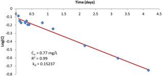
Figure 1. First order regression model of reaction rate constant with initial chlorine residual of 10 mg/L.
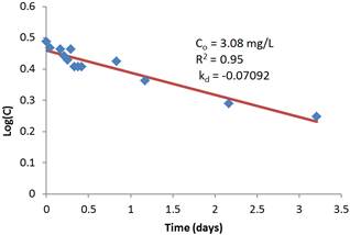
Figure 2. First order regression model of reaction rate constant with initial chlorine residual of 20 mg/L.
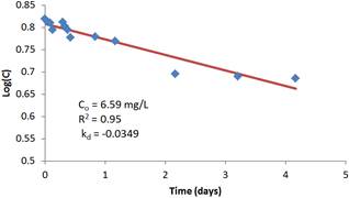
Figure 3. First order regression model of reaction rate constant with initial chlorine residual of 40 mg/L.
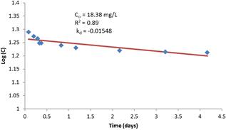
Figure 4. First order regression model of reaction rate constant with initial chlorine residual of 100 mg/L.
Figure 5 also shows that the curve steeps faster at high concentration and the overall slope tends to be flatter when the initial chlorine concentrations are high. Regression analysis with the hypothesized second order rate variation of the decay rate is carried out and the result is superimposed on the linearized plot of the data and shown in Figure 6. It can be seen that the data fit very well this hypothesized model with coefficient of determination (R2 =0.99). The F test results indicate the regression explains the data variation to a confidence level of 99.999% (p = 0.001). The t-test for the slope of the regression line also indicates the significance of the slope being different from zero to a confidence level of 99.999% (P = 0.001).
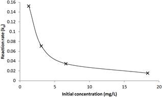
Figure 5. Variation of the bulk decay rate with initial chlorine concentration (model result).
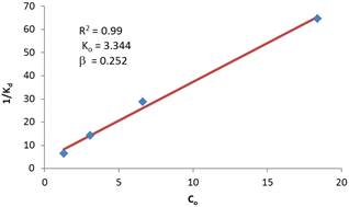
Figure 6. Second order regression model of reaction rate constant with respect to initial concentration of chlorine.
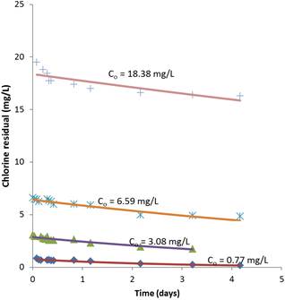
Figure 7. Comparison of second order model prediction of chlorine residual with observed chlorine residuals for different initial chlorine concentrations.
Figure 7 shows the model fits for each of the initial chlorine concentrations used in the experiment. The excellent data fit for the first three initial chlorine concentrations is apparent. The last data with very high chlorine dose (18.38 mg/L) does not fit the data well. This is expected and may be of no practical consequence as chlorine dosages of treated water will not rise to such levels.
The test for normality of the residuals was carried out after the second order chlorine decay rate model was fitted to the data based on the variation of the decay rate with the initial chlorine concentration. The tests that were used to assess normality of the residual are the Q-Q plot and the Shapiron-Wilk test. The SPSS statistical package was used for the tests.
The residual data plot more or less as straight-line on the Q-Q graph. The one outlier for high concentration is apparent though. The Shapiron-Wilk test (Table 1) shows that the probability that the residuals are caused by random variation is 0.44 which is greater than the 0.01 p level of significance needed. The residuals therefore follow normal distribution and the model adequately fits the experimentally determined data.
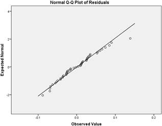
Figure 8. Q-Q plot of residuals (Difference between actual and modeled chlorine residuals).
Table 1. Tests of Normality of residuals (SPSS Output).
| | Kolmogorov-Smirnova | Shapiro-Wilk |
| Statistic | df | Sig. | Statistic | df | Sig. |
| Residuals | .091 | 48 | .200* | .976 | 48 | .442 |
*. This is a lower bound of the true significance.
a. Lilliefors Significance Correction
4. Conclusion
Modelling of chlorine decay in distribution systems is an important exercise for determining the chlorine residuals needed to ensure that required water quality standards are adequately met. Several models commonly in use such as the EPANET require accurate input of bulk decay coefficients that are often experimentally determined.
The theoretical model we built in this research clearly shows that the variation of the bulk decay coefficient with initial chlorine concentrations can be modelled mathematically as a second order reaction. To verify this, experiments were carried out for determining the bulk decay rate of chlorine residuals at different initial chlorine doses. The data obtained fits the proposed second order model adequately. The first order model used in distribution system chlorine residual simulations such as the EPANET can easily accommodate such model as the bulk decay coefficient is adjusted according to the model formula that requires one additional rate parameter describing the effect of initial chlorine concentration. The model that was determined for predicting the effect of initial chlorine concentrations on the chlorine decay rates is also statistically tested to agree well with the observed chlorine concentrations.
It is widely reported that first order modelling may not adequately describe the chlorine decay rate and various attempts have been made to identify and model the effect of several factors that affect the decay rate of chlorine in distribution systems. While the factors are more or less well known and empirical formulae are often proposed, developing a mathematical model or analytical solutions that satisfactorily accommodates such factors is still a challenging problem.
Of the several attempts made in the past to model the variable rate of chlorine decay, the work of Phillip et al. (2009) is important as it tries to accommodate the chlorine concentration, slowest reacting rate and reactant concentrations into an empirical second order model. The solution, however, remains numerical by trial and error besides the model being based on empirical formulations of rate variation.
Our research attempted to develop a mathematical model of the chlorine decay rate further from the work of Phillip et al. (2009) by working around parameters that are difficult to determine such as reaction rates of individual reactants. Two models were developed that were based on time-varied and time-averaged reaction rates while both were concentration-averaged. The models developed are integrated in the sense that one model can be derived as the special or general case of the other. For the time varied model, the parameters affecting the decay rate were found to be the chlorine concentration and the molar concentration of the low concentration reactants as expressed through the ratio of arithmetic mean to the harmonic mean of the reactant concentrations. For the time averaged model that can be used in modelling programs based on first order reactions, the time variation of the rate of reaction was additionally influenced by the aggregate (total) reactant concentrations.
While Phillip et al (2009) emphasized that the reaction rates were being influenced by the rate of reaction of the slow reacting compounds, our model development, however, shows that the molar concentrations of the low concentration reactants do influence the rate of reaction more than the rate of reaction. Additional research work is proposed for developing such models further by taking into account additional factors such as initial react concentration, low concentration reactants and other factors as may be needed.
Acknowledgment
This research study was supported by the government of Finland as part of the Mbabane Dry Sanitation and Waste Management Project (MDSWMP) research activity. The researchers would like to thank the financial assistance provided for carrying out the research work.
References
- Musz, A., Beata Kowalsk, B. and Widomski, K.M. (2009) Some issues concerning the problems of water quality modelling in distribution systems. Ecological chemistry and engineering, 16(S2):175-184.
- Chowdhury, Z. K., Passantino, L., Summers, R. S., Work, L., Smith, N., Rossman, L., et al. (2006). Assessment of Chloramine and Chlorine Residual Decay in the Distribution System. Denver: AWWA Research Foundation.
- Patel, H.M., Goyal, R.V. (2015) Analysis of residual chlorine in simple drinking water distribution system with intermittent water supply. Appl Water Sci., 5:311-319.
- Chawla, V., Prema G. Gurbuxani and G.R.Bhagure, G.R. (2012) Corrosion of water pipes: a comprehensive study of deposits. Journal of Minerals and Materials Characterization and Engineering, Vol. 11, No 5, pp.479-492, 2012.
- Phillip, M., Jonkergouw, R., Soon, T.K., Dragan, S. and Hong, B. (2009). A variable rate coefficient chlorine decay model. Environ. Sci. Technol., 43, 408-414.
- Frias, J., Ribas, F., and Lucena, F. (2001) Effects of different nutrients on bacterial growth in a pilot distribution system, Antonie van Leeuwenhoek, 80, 129-138, 2001.
- Hallam N.B., West J.R., Forster C.F., Powellb J.C., Spencer I., (2002). The decay of chlorine associated with the pipe wall in water distribution systems. Water Research; 36(14), 3479-88.
- Mays, L.W. (2000). Water Distribution System Hand Book. Mc-Graw Hill, New York, USA.
- Mahrous, Y.M., Abdullah S., Al-Ghamdi, A., Elfeki, A.M.M. (2015)Modelling chlorine decay in pipes using two-state random walk approach. International Journal of Engineering and Advanced Technology (IJEAT), 4(3):110-115.
- Rossmann, L.A., Clark, R.M and King, L.M. (1994).Modelling Chlorine Residuals in Drinking-Water Distribution Systems. Journal of Environmental Engineering, 120(4): pp. 803-820.
- Jamwal, P., Naveen, M.N., and Javeed, Y. (2015) Estimating fast and slow reacting component in surface and groundwater using 2R model. Drink. Water Eng. Sci. Discuss., 8, 197-217.
- Sonia, A.H. and Istvan, L. (2015) Influence of water quality characters on kinetics of chlorine bulk decay in water distribution systems. International Journal of Applied Science and Technology, Vol. 5, No. 4; 64-73.
- Fisher, I., Kastl, G., and Sathasivan, A. (2011) Evaluation of suitable chlorine bulk-decay models for water distribution systems, Water Res., 45, 4896-4908.
- Clark, R.M. (1998) Chlorine demand and TTHM formation kinetics: a second-order model, J. Environ. Eng., ASCE, 124(1), pp. 16-24.
- Jadas-Hecart A., El Morer A., Stitou M., Bouillot P., Legube P. (1992) Modelisation De La Demandeen Chlore D’une Eau Traitee, Water Research, 26(8), pp. 1073.
- Ventresque C.,Bablon, G., legube, B., Jadas-Hecart, A., Dore, M. (1990). Development of chlorine demand kinetics in drinking water treatment plant, Water chlorination: Chemistry, environmental impact and health effects, R.L. Jolley et al. (1990). Vol. 6, Lewis Publications, Inc, Chelsea, MI, pp. 715-728.
- Dharmarajah Hatania N. (1991) Empirical modelling of chlorine and chloramine residual, AWWA Proceedings: Water Quality for the New Decade, Annual Conference, Philadelphia, PA, pp. 569-577.
- Hua F., West J.R., Barker R.A., Forster C.F. (1999) Modelling of chlorine decay in municipal water system. Water Research, 1999, 33(12), pp. 2735-2746.
- Vasconcelos J.J., L.A. Rossman, W.M. Grayman, P.F. Boulos, and R.M. Clark. (1996) Characterization and modelling of chlorine decay in distribution Systems. AWWA Research Foundation. ISBN: 0-89867-870-6. Denver, CO.
- Powell J.C., Hallam N.B., West J.R., Forester C.F., Simms J. (2000a) Factors which control bulk chlorine decay rates. Water Res 34(1):117-126.
- Powell J.C., West J.R., Hallam N.B., Forster C.F., Simm J. (2000b) Performance of various kinetic models for chlorine decay. J Water Resour Plan Manag ASCE 126(1):13-20.
- Vieira, P., Coelho, S.T., Loureiro, D. (2004). Accounting for the Influence of Initial Chlorine Concentration, TOC, Iron and Temperature When Modelling Chlorine Decay in Water Supply. Journal of Water Supply: Research and Technology-AQUA 53 (7), 53-467.
- Hallam, N. B.; Hua, F.; West, J. R.; Forster, C. F.; Simms, J. (2003) Bulk decay of chlorine in water distribution systems. J. Water Res. Plann. Manage., 129, 78-81.
- Boccelli, D. L.; Tryby, M. E.; Uber, J. G.; Summers, R. S. (2003) A reactive species model for chlorine decay and THM formation under rechlorination conditions. Water Res., 37, 2654-2666.
- Kastl, G., Fisher, I., Jegatheesan, V. (1999). Evaluation of chlorine kinetics expressions for drinking water distribution modelling. Journal of Water Supply: Research and Technology. Aqua 48 (6): 219-226.
- APHA (1999) Standard Methods for the examination of Water and Wastewater: Chemical Oxygen Demand, 5220, # (102). American Public Health Association, American Water Works Association, Water Environment Federation.


