K Meson Decays in Quark Model

Kh. Ghasemi¹, N. Ghahramany², H. Mehraban¹

¹Islamic Azad University, Central Tehran Branch, Tehran, Iran

²Islamic Azad University, Arsanjan Branch, Arsanjan, Iran

Email address

Citation

Kh. Ghasemi, N. Ghahramany, H. Mehraban. K Meson Decays in Quark Model. International Journal of Modern Physics and Application. Vol. 3, No. 3, 2016, pp. 45-51.

Abstract

In this paper, the decay of  mesons have been studied by means of the Effective Hamiltonian Theory. Decay rates of the constituent S and  quarks, in the tree and penguin levels are calculated via effective Lagrangian density of the weak interaction and then by using these obtained decay rates, the decay rates and branching ratios of K and  are calculated and compared with the experimental results. Findings from this study are in a good agreement with the experimental values.

Keywords

K Meson, Quark Model, Effective Hamiltonian, Branching Ratio, Decay Rate

1. Introduction

One of the successful models in particle phenomenology is the quark model which is applied to calculate the decay rates of various particles. The particles called kaons, were first observed in late 1940s in cosmic-ray experiments. By today’s standards, they are common, easily produced, and well understood. Over the last four decades, studies on how kaons decay have played a major role in development of the Standard Model. Yet, after all this time, kaon decays may still prove to be a valuable source of new information on some of the remaining fundamental questions in particle physics.

When first observed, kaons seemed quite mysterious. Experiments showed that they were produced in reactions involving the strong force, or strong interaction – the most powerful of the four fundamental forces in nature – but they did not decay (that is, transform into two or more less massive particles) through the strong interaction. This is due to kaons retaining a feature which ultimately labeled "strangeness," that is conserved in the strong interaction [1].

One of the most interesting and unique observed particles in the nature is kaon. There are two neutral kaons which are, in fact, strange mesons.

                                             (1-1)

 is the eigenvalue of the strange state. Since each kaon under CP effect turns into another kaon, neither of these kaons have determined CP number.  and  are not eigenstate of CP. However, when CP acts on them, they are conjugate of each other.

                                                 (1-2)

But theorists can make a pair kaon with determined CP from combination of wave

function and . According to Quantum Mechanics rules, these combinations correspond with real particles and have a mass and determined lifetime. Therefore normalized eigenstate CP are [2, 14]:

                   (1-3)

So,

             (1-4)

 can just decays to  state, while  should go to  state. Neutral kaons usually decay to two or three pions. Arrangement of two pions has +1 parity and three pions system has -1 parity and both of them have a. As a result,  decays to two pions and  decays to three pions [3].

                            (1-5)

Since a kaon has hardly enough mass to produce three pions, two pion decays are fast but three pion decays are longer. Observed lifetimes are about  and, respectively [2, 10].

 meson decay, as a weak decay, in the presence of strong interactions requires a special approach. The main tool to investigate these decays is the effective Hamiltonian Theory. Beginning of any phenomenological weak decay of hadrons is the effective weak Hamiltonian. Its structure is as follows:

                  (1-6)

Where  is the Fermi constant represented in terms of the weak coupling constant and  boson mass is defined as follows:

 =                          (1-7)

And are the local operators which control the decay. , the Cabibbo–Kobayashi–Maskawa factors and , the Wilson ‍Coefficients are described by the force with which an operator enters the Hamiltonian. In fact, the effective point-like vertices are represented by local operators that can correct the picture of the decay of hadrons with a mass of the order of  a better way to provide.  The Wilson coefficients to be used as coupling constants (depending on scale) corresponding to the vertices are taken into account. Selection of the  scale is optional, but it is customary to choose  from the order of the mass of hadrons decaying, e.g forandmesons decay, the value of  are in the order of  and , respectively. For kaon decays, the common choice of  is in the order of  instead of  order [4].

2. Calculation of  Decay Rates in the Tree Level

The standard model can be used for those particle decays in which their non- perturbative aspects, mainly do not affect the decay process. In fact here, the modes of S quark decays are studied which have not entered the QCD area and take place by bosons. This area is called the tree level [2].

Effective Lagrangian density related to the weak interaction could be expressed in terms of the coupling of the weak currents. Since the  decays through particle in tree level is being investigated here, the weak currents in Lagrangian, the charged currents and Effective Lagrangian density, could be described as following [5, 6]:

                            (2-1)

Assuming that the wave functions of particle and antiparticle are normalized in  volume, with the coefficient of normalization of , and assuming that the quark is at rest (), the currents in above equation is given as follow:

        (2-2)

Here , so,  that  are the Pauli  matrices, also  is the identity matrix. Furthermore,  and are the elements of the  matrix. Assuming  (quark's momentum in x-z plane) the positive and negative helicity of the quarks could be expressed as follows:

                             (2-3)

According to the Perturbation Theory, the decay matrix element in the lowest-order is [7]:

                       (2-4)

However, substituting  in Eq. (2-4), then:

  (2-5)

In which with considering relations of quarks speed,  is defined:

                                            (2-6)

Now in order to calculate the decay amplitude, the  components for and over the quark spin states  and, are found. The spin average sentence is:

                                          (2-7)

The above relation is obtained for final quarks in) helicity state. There are 8 helicity states. All of the helicity states are summed.

           (2-8)

The decay rate is:

     (2-9)

Where,

 and .

With considering that the angle between velocity of particles must be physical, , in that result:

                      (2-10)

If Eq. (2-5) is substituted in Eq. (2-9) and perform the calculations, then:

                  (2-11)

Where  is the phase space integral and .

The important point here is that it is assumed, the color factor to be 3 for Hadron decays. The decay rate for semi-lepton decays (assuming that the matrix elements of the lepton vertices are considered to be equal to 1) and the Hadron decays are:

                         (2-12)

                   (2-13)

Table 1 presents the decay rate with corresponding errors in tree level for several numbers of semi-lepton and hadron decays of S quark, respectively, by using Eqs (2-12) and (2-13). The sources of errors correspond to quark mass data taken from [9].

Table 1.  Quark Decay Rate in Tree level.

3. Calculation of the  Decay Rates in Tree and Penguin Levels

In the standard model, Flavor Changing Neutral Current () is prohibited. For example, there is no direct coupling between the quark and the  and quarks. In fact, at the vertices of the ،  and neutral boson, the quark flavors do not change. This fact indicates the absence of currents in the tree level.

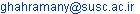
 vertices could be used in building up the desired structure of the loops. In another words,  currents are created by penguin or one-loop diagrams. A penguin diagram and the schema of the Penguin are presented in Figure 1:

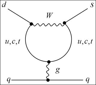
Figure 1. Penguin level.

As it could be observed in Figure 1, one loop is created. In fact, in this loop, for example, a boson is emitted during the decay, while  quark is converted to the internal quark. Then the boson is absorbed and  quark is converted to quark. So Penguin diagrams contain a - bosons - quarks loop. It could be seen that the  transition in  decay in figure 2.

Figure 2.  Transition in  decay in penguin level.

Different types of penguin processes include Electromagnetic Penguin, Electroweak Penguin and Gluons and QCD Penguin. The gluon penguins in which from Penguin’s loop a gluon is emitted and it will generate a quark and anti-quark will be examined. Since the flavor of quark remains constant in gluon coupling, the Penguins could not be produced in the  decay, by the  operator (which represents  and operators of the decays in the tree level). Therefore, the Hamiltonian in the presence of additional interactions in penguins becomes more complicated; consequently, the new operators enter.

The Effective Hamiltonian in the Tree and Penguin level is given as [13]:

                    (3-1)

Where,  are the current-current operators and  are the gluon penguin. For  decay, coefficients are:

                      (3-2)

And as it is already known,  are the Wilson coefficients. It is required to find all helicity states, for ،...،, and then sum up.

              (3-3)

It is necessary for calculating all helecity states, ،...،. The helicity states include:

           (3-4)

We know that the helicity states ،...، are proportional with terms and the helicity states , are proportional with terms. Therefore,

 (3-5)

Where, ,  and  are defined as follows:

                                 (3-6)

Decay rate is:

                                     (3-7)

                    (3-8)

                            (3-9)

Where, ,  and  are the phase space integrals.

The general framework to obtain the Wilson coefficients is similar to what was mentioned in Eq (1-6). Therefore, the effective Hamiltonian of the  transition is defined as follows [7]:

  (3-10)

Where  is the Fermi constant and  are the local operators which control the decay.  coefficients are the Wilson ‍Coefficients. The overall structure of the Wilson coefficients is as follow [12]:

                       (3-11)

In this equation  is defined as follows:

                                 (3-12)

To obtain quark decay rate, the effective Wilson coefficients of the tree and penguin decay is needed. The effective Wilson coefficients could be defined as follows [7]:

                (3-13)

Table 2 presents the calculated values for the Wilson coefficients of the  quark and  anti-quark decay.

Table 2. The effective Wilson Coefficients at the Renormalization Scale.

 quark and  anti-quark decay rates in tree and penguin level by the use of effective Hamiltonian theory are presented in table 3.

Table 3.  Quark and  Anti-Quark Decay Rates in Tree and Penguin Level.

4. Calculation of Branching Ratio

As it is known, most of the particles could decay in many different ways. For  decay modes, the branching ratio is defined as follows:

                             (4-1)

The branching ratio of the quark decay mode is defined as, quark decay rate of each mode to the summation rates of semi-lepton and non-lepton decays. For example, there is:

                    (4-2)

Where  is the summation of semi-leptonic transition and  is the non-leptonic transition. The total decay rate is given by:

We observe  Quark and anti-quark decays, branching ratios that are calculated and summarized in Table 4 in which the  and  values are taken from tables 1 and 3, respectively. These calculated values are compared with experimental  values for  mesons decays, related to, ,  and  transitions. Through comparison, it could be concluded that the theoretical values are in good agreement with the experimental values.

Table 4. Experimental Values of the Branching Ratio of SeveralMeson Decays and Comparison with Theoretical Values.

Table 5. Theoretical Values for the CP Violation in  Quark Decays.

Now applying the asymmetric relationship:

                      (4-3)

And by using  values listed in Table 3, violations are calculated. Results are presented in Table 5.

5. Conclusion

By using the effective Lagrangian density of the weak interaction,  decay rate is calculated in tree level. Furthermore, decay rates of S quark –anti quark are calculated in tree and penguin level by the use of the effective Hamiltonian Theory.

Comparison between  Values in Table 3 and the results in Table 1 shows that the penguin contributions in the quark decays are small.

Comparing the S quarks decay branching ratio without non-perturbative inclusion in table 4, it could be concluded that findings from this study are in a good agreement with the experimental values.

Considering Table 5, it could be realized that, since  and  are not anti-symmetric, the  violation does not happen. In  decays,  conservation is observed, which is in agreement with experiment given in reference [11].

References

1. J.Ritche "Rare kaon decays" BEAM LINE, V.25, N.4, (1995).
2. K.Lande et al.,Phys. Rev. 103, 1901(1956).
3. Griffihs, D.J., "Introduction to Elementary Particles", John Wiley & Sons (1987).
4. Andrzej J.B., "Operator Product Expansion, Renormalization Group and Weak Decays", Lect. Notes. Phys. 558, pp.65-85 hep-ph/9901409 TUM-HEP-343-99. (2000).
5. Cottingham, W.N., Greenwood D.A., "An Introduction to The Standard Model Of Particle Physics", Second Edition, University of Bristol, UK (2001).
6. Buchalla, G., Andrzej J.B., Lautenbacher, M.E., "Weak Decays Beyond Leading Logarithms", Rev. Mod. Phys., 86, 4 (Oct 1996).
7. Cheng, H.Y., "The  Rule In Kaon Decays", Chinese Journal Of Physics, 38, 4 (2000).
8. Cheng, H.Y., "Factorization Approach For The  Rule and  In Kaon Decays", Chin. J. Phys., 38, (2000).
9. Amster, C., "Particle Data Group", PLB667 (2008),J. Beringer et al. (Particle Data Group), PR D86, 010001 (2012).
10. Halkiadakis, E., "Measurements ofNeutral Kaon Decays To Two Electron-Positron", University of New Brunswick, New Jersey (May 2001).
11. Sakurai.J.J, "Modern Quantum Mechanics", (Revised Edition), (10 September 1993).
12. V. Cirigliano, G. Ecker, H. Neufeld, A. Pich and J. Portol´es, "Kaon Decays in the Standard Model", Rev. Mod. Phys. 84, 399 (2012).
13. H.Mehraban, "Effective Hamiltonian and Effective Penguin Model on b Quark Decays", Transaction B: Mechanical Engineering, Vol. 16, No. 5, pp. 371{386}, (2009).
14. K. K. Vos, J. P. Noordmans, H. W. Wilschut and R. G. E. Timmermans1, "Exploration of Lorentz violation in neutral-kaon decay", phys. letter B 729, 112, (2014).
15. A.Baratt. Ph.D. thesis, "Branching Ratios of the Charged Kaon Decays and Radiative Corrections for the Decay Mode", University of Pittsburgh, (2004).
16. T. K. Komatsubara, "Experiments with K-Meson Decays", arXiv: 1203.6437v1, (29 Mar2012).
17. J.Bijnens, "Weak Introduction of Light Flavors", arxiv: hep-ph/0010265v1, (2000).