-Least Square Support Vector Method for Solving Differential Equations

Mojtaba Baymani^{1, *}, Omid Teymoori¹, Seyed GHasem Razavi²

¹Department of Computer and Mathematics, Quchan University of Advanced Technology, Quchan, Iran

²Department of Mathematics, Ferdowsi University of Mashhad, Mashhad, Iran

Email address

^*Corresponding author

Citation

Mojtaba Baymani, Omid Teymoori, Seyed GHasem Razavi. -Least Square Support Vector Method for Solving Differential Equations. American Journal of Computer Science and Information Engineering. Vol. 3, No. 1, 2016, pp. 1-6.

Abstract

In this paper, a new method based on -Least Square Support Vector Machines (-LSSVM’s) is developed for obtaining the solution of the ordinary differential equations in an analytical function form. The approximate solution procedure is based upon forming of support vector machines (SVM’s) whose parameters are adjusted to solve a quadratic programming problem. The details of the method are discussed, and the capabilities of the method are illustrated by solving some differential equations. The performance of the method and the accuracy of the results are evaluated by comparing with the available numerical and analytical solutions.

Keywords

Ordinary Differential Equation, -Least Squares Support Vector Machine, Quadratic Programming Problem, Constrained Optimization Problem

1. Introduction

We consider the m-th order linear ODE by initial conditions as follows:

              (1)

                  (2)

where ,  are the given functions,  is the given scalar and  denotes the i-th derivative of function y(t) with respect to .

Nowadays, Many of the problems in studies fields; including engineering, medical sciences and medicine can be applied to a set of differential equations (DE’s) through a process of mathematical modeling is reduced. Because in most cases it is not easy to get the exact solution of DE’s, so numerical methods should be applied. There are a lot of mathematical methods to solve DE’s. Most techniques offer a discrete solution such as finite difference (for example predictor-corrector, or Runge-Kutta methods) or a solution of limited differentiability (for example finite elements). These methods define a mesh (domain discretization) and functions are approximated locally ([1]-[2]).

Recently, researchers proposed some new methods that were based on artificial neural network (ANN) models. The ANN methods in comparison with other numerical methods have more advantages. The solution of DE’s in ANN methods are differentiable and continuous ([3]-[5]). Lagaris et al. [3] used neural networks to solve ODE’s and PDE’s. They used multilayer perceptron in their network architecture. Malek et al. [4] proposed a novel hybrid method based on optimization techniques and neural networks methods for

the solution of high order ODE’s. They offered a new solution method for the approximated solution of high order ODE’s using innovative mathematical tools and neural-like systems of computation. Fasshauer [6] proposed a new unsupervised training method by using Radial Basis functions (RBF) to solve DE’s. The methods based on genetic programming have also been proposed as well as methods that induce the underlying differential equation from experimental data. The technique of genetic programming is an optimization process based on the evolution of a large number of candidate solutions through genetic operations such as replication, cross over and mutation ([7]-[9]).

Recently Suykens and Mehrkanoon proposed approximating solutions to ODE’s and PDE’s using LSSVM’s model. Also, they are extended them approaches in approximate solution to linear time varying descriptor systems ([13]-[14]).

In this paper, we introduce a new method based on SVM’s for solving DE’s. SVM’s are very popular methods in machine learning which solving pattern recognition and function estimation problems ([10]-[12]). We will utilizing -LSSVM [15] method for solving ODEs. In last section will show that our results have better accuracy and loss error.

2. -LSSVM for Regression

We consider a given training set  with input data  and output data. The regression problem is to estimate a model of the form . The primal problem of -LSSVM regression is follow:

          (3)

According to [15], the dual problem of (3) is

        (4)

where  is a given positive definite function (kernel function). We use the following differential operators in next section which employed in [13]:

.

3. Description of the Method

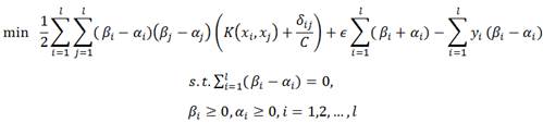
To obtain a solution of (1) the collocation method is adopted which assumes a discretization of the interval  into a set of collocation points (training points). Let  denote the approximate solution to (1), with adjustable parameters  and , the problem (1) is transformed to the following quadratic programming problem:

s.t.

                  (5)

In practice, the quadratic programming problem (5) is solved via its dual.

Lemma: The solution to (5) is obtained by solving the following the quadratic programming problem:

                                 (6)

where

where,  and .

Proof: The Lagrangian of the constrained optimization problem (5) becomes

where ,  and  for  are Lagrange multipliers and  and  are slack variables. Then, optimality conditions are as follows,

We are imposing  and then dual of (6) are as follows:

       (7)

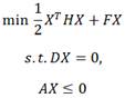
If using the following matrix form for problem (7), we can give the Dual problem (6),

.

The obtained approximation solution is as follows,

4. Numerical Results

In this section, we used the performance of the approach methods on two problems, first order and second order IVP. Therefore we solved two problems with -LSSVM model and then compared by SVM and LSSVM models [13] to shows that which of them are better. For all the problems, the RBF kernel is used (). Also, we use the set of midpoints of training points () as test point and compute the mean squared error (MSE) for the validation:

MATLAB 2015a is used to implement the code and all computational were carried out on a windows 8 system with Intel Pentium- ULV, 1.8 GHz CPU and4.00 GB RAM.

Example 1. Consider the following first order IVP [5]:

Exact solution of this example is

The approximate solution by the proposed -LSSVM method are compared with the analytic solution; also we are compared numerical results of -LSSVM, SVM and LSSVM methods with together where are shown in Table 1. In this example, we suppose ,  and  for different amounts . The results of this example shows that -LSSVM method for any  is the best method to relieve high accuracy and SVM model is not good; because, for  give to us the high error amounts and is not suitable. Also in Fig. 1 the error function  for  and 100 is depicted which shows the solution is very accurate

Table 1. The comparison of our proposed method with SVM and LSSVM methods for example 1.

Example 2. Consider the following second order IVP [3]:

The exact solution of this example is

Table 2. The comparison of our proposed method with SVM and LSSVM methods for example2.

The approximate solution by the proposed -LSSVM method are compared with the analytic solution; also we are compared numerical results of -LSSVM, SVM and LSSVM methods with together where are shown in Table 2. In this example, we suppose ,  and  for different amounts . This Table shows that -LSSVM method for any  is the best method to relieve high accuracy and SVM model is not good; beacuse, for  give to us the high error amounts and is not suitable. Also, error amounts for any  in LSSVM is losser -LSSVM. But, for  results not continues an antiseptic process. In Figures 2 the error function  is depicted which shows the approximate solution convergence to exact solution. Also, In Figures 3 the error function ) is depicted which shows the approximate solution is differentiable.

5. Conclusion

In this paper a new method based on -LSSVM has been applied to find solutions for m-th order differential equations with initial conditions. The solution via -LSSVM method is a differentiable, closed analytic form easily used in any subsequent calculation. The neural network here allows us to obtain the solution of differential equations starting from training data sets and refined it without wasting memory space and therefore reducing the complexity of the problem. If we compare the results of the numerical methods with our methods, we see that our method has some small error. Other advantage of this method, the solution of differential equation is available for each arbitrary point in training interval (even between training points).

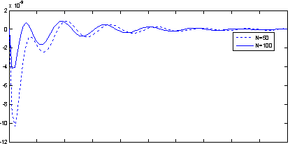
Fig. 1. The error function ) for example1 when [0; 10] is discretized into 50 and 100 equal parts.

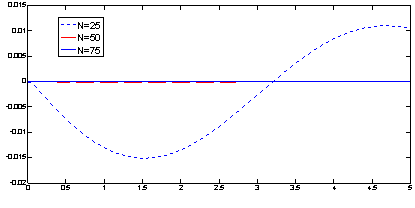
Fig. 2. The error function ) for example 2 when [0; 5] is discretized into 25, 50 and 75 equal parts.

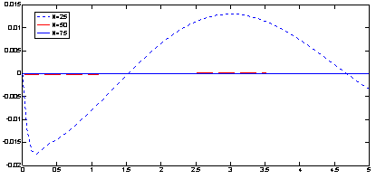
Fig. 3. The error function ) for example2 when [0; 5] is discretized into 25, 50 and 75 equal parts.

Acknowledgements

This work was supported by Quchan University of Advanced Technology under grant number 1024.

References

1. S. D. Conte, C. de Boor, "Elementary numerical analysis, an algorithmic approach", Third Edition, 1980.
2. D. R. Kincaid, E. W. Cheney, "Numerical analysis mathematics of scientific computing",third ed., Brooks/Cole, Pasific Grove CA, 2002.
3. I. L. Lagaris, A. Likas, D. I. Fotiadis, "Artificial neural networks for solving ordinary and partial differential equations",IEEE Transactions on Neural Networks, 9(5), 987-1000(1998).
4. A. Malek, R. Shekari Beidokhti, Numerical solution for high order differential equations using a hybrid neural network optimization method, Applied Mathematics and Computation 183, 260-271(2006).
5. H. S. Yazdi, M. Pakdaman, H. Modaghegh, Unsupervised kernel least square algorithm for solving Ordinary Differential Equations, Neurocomputing 74, 2062-2071, (2011).
6. G. E. Fasshauer, Solving Differential Equations with Radial Basis Functions: Multilevel Methods and Smoothing, Advances in Computational Mathematics, 11(2), 139-159(1999).
7. G. Burgess, Finding Approximate Analytic Solutions to Differential Equations Using Genetic Programming, Surveillance Systems Division, Electronics and Surveillance Research Laboratory, Department of Defense, Australia, 1999.
8. I. G. Tsulos, I. E. Lagaris, Solving differential equations with genetic programming", Genetic Programming Evolable Machines, 7, 33-54(2006).
9. J. R. Koza, Genetic Programming: On the programming of Computer by Means of Natural Selection. MIT Press: Cambridge, MA, 1992.
10. V. Vapnik, "Statistical learning theory", New York: Wiley (1998).
11. V. Vapnik, "The natural of statistical learning theory", Springer New York (1995).
12. Y. Xu, X. Pan, Structural least square twin support vector machine for classification, Springer Science and Business Media New York, 42, 527-536(2015).
13. S. Mehrkanoon, T. Flack and J. A. K. Suykens, Approximate solutions to ordinary differential equations using least squares support vector machines, IEEE Transactions on Neural Networks and Learning Systems 23, 1356-1367(2012).
14. S. Mehrkanoon, J. A. K. Suykens, LS-SVM approximate solution to linear time varying descriptor systems", Automatica, 48, 2502-2511(2012).
15. Y. J. Tian, X. C. Ju, Z. Qi and Y. Shi, Efficient sparse least squares support vector machines for pattern classification, Computers and Mathematics with Applications 28(6), (2013).
16. J. A. K. Suykens and J. Vandewalle, Least squares support vector machine classifier, Neural Processing Letters 9(3), 293-300(1999).
17. D. Tax and R. Duin, Support vector domain description, Pattern Recognition Letter 20, 1191-1199(1999).
18. D. Tax and R. Duin, Support vector data description", Machine Learning 54, 45-66 (2004).