Residential Lighting Load Profile Predictor Using Computational Intelligence
Olawale M. Popoola
Centre for Energy and Electric Power, Department of Electrical Engineering, Tshwane University of Technology, Pretoria, South Africa
Email address
Citation
Olawale M. Popoola. Residential Lighting Load Profile Predictor Using Computational Intelligence. American Journal of Energy and Power Engineering. Vol. 3, No. 2, 2016, pp. 10-18.
Abstract
This study presents the development, analysis and assessment of residential lighting load profile using computational intelligence based modelling - Adaptive Neuro Fuzzy Inference System (ANFIS) and Neural network (NN) models for prediction (forecasting) and evaluation of lighting load and initiatives. Factors considered in the development of the models include natural lighting, occupancy (active) and income level. Trapezoidal membership and sigmoid transfer function were applied during the training process of the ANFIS-based and NN-based model respectively. Using computational and different validation approaches, ANFIS gave better correlation and error level results in comparison with the NN-based method analyses notably morning standard, morning / evening peak and daily TOU (time of use) periods. The inference attribute of the ANFIS model based on characterization factors and its reflection of occupants’ complexity on lighting loads in residential buildings makes it a better lighting predictor especially in demand side management & residential lighting load energy efficiency project initiatives.
Keywords
Energy, Computational Intelligence, Simulation Model Technique, Statistical Analysis, Demand Profile Forecasting
1. Introduction
Electricity demand outstripping generation has been shown by recent events around developing countries. Hence the need to institute different ways of coping with such issue i.e. using energy reduction, demand side management, implementation of energy technologies’, etc. According to the research carried by Pike research (2010) governments and organizations have looked to "lighting" as a swift means of achieving energy reduction [1]. A fifth of the total electricity consumption in an average household represents lighting demand [2]. Incentives and other programs to encourage and guide developers to implement efficient lighting in existing facilities and new projects has been put in place in South Africa and some other countries. This may has been deduced from research findings such as work carried out carried by Wong et al, 2010 which showed that lighting accounts for 20-30% of electricity consumption in a building [3]. Most impact evaluation of lighting usage / technologies has been based on fixed conditions where the presence of people and interactions of people are handled in an entirely deterministic way including some simulation programs. Other practices adopted at present in modelling lighting load in residential homes, do not reflect the complexity of the occupant(s) behaviour and the impact of environmental factors on such buildings and behaviour. Categorised methods or techniques that have been used for prediction or estimation of energy usage and lighting load includes statistical methods, analytical methods, empirical methods and modelling methods [3]-[12].
As a result of human beings unpredictability, consumption habits, social lifestyle and cost of metering, lighting load model development have been relatively studied. This may be as a result of electricity consumption being inevitably influenced by random factors, while demand time series experiences highly non-linear characteristics [6]. Some of this factor-s can be introduced to contribute and improved the prediction and estimation of lighting load within the residential sector. These factors may include occupant presence and effect on light usage, comfort level and income of individuals, location of residences and areas in terms of daylight effect, demographics characteristics etc. Literature discussions have shown that human behaviour and environmental climate could significantly change lighting usage in a residential dwelling within a period e.g. monthly or yearly basis [2]-[7]-[11]-[20].
Having this as a background, an approach that is capable of such characterization i.e. non-linearity, variableness, uncertainty and the ability to learn from historical data is needed. Adaptive network-based fuzzy inference system (ANFIS) is one of such approach. Studies using ANFIS for good predictability include, forecasting the amount of water discharge by stream water (River Kaduna) [13], prediction of surface roughness in turning operation [14], prediction model for water reservoir management [15] and river flow estimation by [16]. Result obtained showed that the ANFIS model is capable of high prediction accuracy. Another study using ANFIS approach was forecasting regional electricity loads. The study showed that ANFIS model has a better forecasting performance in comparison to the regression model, support vector machines with genetic algorithms, artificial neural network (ANN) model, recurrent support vector machines with genetic algorithms (RSVMG) model and the hybrid ellipsoidal fuzzy systems for time series forecasting (HEFST) model [17]. Another work carried out using ANFIS in combination with radial basis function (RBF) neural network was in the real-time price environment for the electricity market. The authors were able to demonstrate the flexibility and practicality of the model under the environment [18].
The main purpose of this study is to present an ANFIS based model lighting load predictor, assess and compare its performance with a learning algorithm based model (Neural network) for middle-income residential group.
The outline of the study consists of the network structure, the parameter estimating algorithms, description of the main study group (middle-income earners), available data, model process design and strategy / development. Lastly, the discussion of models result, performance assessment and impact evaluation is carried out.
1.1. Adaptive Neural Fuzzy Inference System (ANFIS)
ANFIS well suited to mathematical analysis can simply be defined as a set of fuzzy 'if–then' rules with appropriate membership functions to generate the stipulated input–output pairs in the solution of uncertain and ill-defined systems [19]. The fuzzy inference is the process of formulating the mapping from a given input to output using fuzzy logic. The mapping then provides a basis from which decisions can be made or pattern discerned. The process of fuzzy inference involves membership functions, fuzzy logic operators, and if-then rules. This procedure (Fig. 1) is used to compute the mapping from the input values to the output values, and it consists of three sub-processes, fuzzification, aggregation, and defuzzification. Backward propagation algorithms and hybrid-learning algorithms methods are use for determination of the membership functions, learning provision of the ANFIS and construction of the rules. In general ANFIS system has input layer, output layer, and hidden layers that represent membership function and fuzzy rules. A typical three rule systems is shown as follows:
Rule 1: if  is A1,
  is B1 and
  is C1, then

Rule 2: if x is A2, is B2 and z is C2, then

Rule 3: if x is A3, is B3 and z is C3, then

General rule being

Where x, y and z represents our inputs which are fuzzy sets Ai, Bi, and Ci representing natural lighting, occupancy and income. p, q, and z are the design parameters that will be determined during the training process.
1.2. Feed Forward Back Propagation Neural Network (FFNN)
The back propagation neural network consists of input layer, output layer, and hidden layers of neurons. Each layer has numerous neurons; each neuron is interconnected with adaptable weighted connections to neurons in the subsequent layer. The process of training involves the tuning of weights in order for the network to produce the desired output in relation to the particular inputs. To minimize the error function in relation to the desired output and actual FFNN outputs, a two-layer feed forward network and Levenberg-Marquardt back propagation learning algorithms is employed for this study.
Fig. 1. ANFIS mapping.
1.3. Model Development Design Strategy
Fig. 2 shows the model development strategy applied. This entails relationship exploration based on characterization factors for model development that captures the non-linearity and complexities associated with residential lighting usage. Three input factors namely natural light level, effective occupancy (Active/Awake occupancy) and household income grouping will be applied. The design strategy involves interactive importing and exploration of files, query of databases, filtrations and categorization of data feeds, use of Matlab / Excel sheet or interactive data language.
Fig. 2. Logic Lights Usage Output Design.
2. Study Methodology and Material
ANFIS & NN techniques were applied to model a middle-income earner 24 hour lighting usage profile in a locality in Gauteng province, South Africa. Three input variables natural lighting (irradiance level), occupancy (active), and income earning are considered in relation to environmental factors, daily activities and its social class within the society. A survey data of 102 buildings carried out within the locality in the year 2010 as the input variables were used for both training and checking database (70%: 30% ratio). The classification of data as "error free" is because of the performance tracking exercise (physical audit and telephonic exercise) conducted periodically (yearly) to ascertain the impact of the utility compact fluorescent rollout. This conforms to the international performance measurement and verification protocol. The survey data are mainly historical obtained during the Eskom Measurement &Verification Compact Fluorescent initiative (CFL) implemented in the country using physical door to door exercise. The questionnaires format included the following key points: (i) Daily wake up time; switching ON lights and room involved; (ii) Occupant(s) departure time - from home; (iii) Time the occupant returned back home; (iv) Food preparation time and room lights that are ON in the evening; (iv) Sleeping time, (v) Bathing time (morning and /or evening). The information gathered will be interpreted using 0 and 1 format. This will then be weighted between 0 and 1 using an average weight per household utilization. Further validation of the model entailed the use of logging database (occupancy and lighting switch ON-OFF event) for a month period (November 2013 to April 2014) in homes for the various income groups and the use of different household’s survey profile data (Popoola et al., 2015).
2.1. Metering
For the metering aspect, Onset Hobo UX90-005/-006 or UX90-005M/-006M loggers were attached to each indoor luminaries or set of luminaries, on separate switch at the residential dwellings. One-minute resolution was used to capture the peaks and short duration events in this study. The data was downloaded and interpreted using the same format interpretation as the survey data.
2.2. Sample Size
The sample size is governed by confidence level - the level of certainty that the characteristics of the data collected will represent population characteristics; the margin of error that can be tolerated; statistical technique and analysis to be undertaken and lastly the size of the total population from which our sample is being drawn. This investigation was carried out using data sample size of 125 within the locality, however due to incomplete information, only 102 buildings were used for this investigation.
3. Metering and Investigation Analysis
3.1. Occupancy
Most dwellings were occupied during the evening period as shown by the result obtained from the data loggers installed in different rooms within household dwellings in relation to average lighting usage and occupancy, while there was little or no occupancy during the daytime (Popoola et al., 2015). The findings were collaborated by the historical survey questionnaires. Other deductions include sharing of lighting especially in the evening and; increase and decrease in room occupancy at certain TOU due to varying factors (Popoola et al., 2015).
The assigned weights to reflect the active occupied room within the dwelling, which is expected to be variable throughout the day, is shown in Table 1. This is expected to contribute to effectual determination of the power demand at specific intervals.
Table 1. Rooms occupancy weights.

3.2. Natural Lighting
A correlation coefficient of r = - 0.432116 was obtained from equation 1 based on data acquired from Hobo loggers (Popoola et al., 2014-Sims). The negative result obtained shows that an inversely proportional relationship exists between the switch ON (x) and switch OFF (y) event of artificial lighting. This thereby demonstrates that natural lighting plays a vital part in the use of artificial lighting usage.
 (1)
(1)
where: 
x = switch ON event; y = switch OFF representing high natural lighting irradiance
To simplify the investigation further, natural lighting was assigned weights also. Different weights were assigned according to the level of natural lighting (irradiance level) within 24-hours period in South Africa as follows: No Natural lighting = 0; Natural Lighting low = 0.3; Natural Lighting medium = 0.7 and Natural Lighting high = 1(Popoola et al., 2015).
3.3. Income
Due to occupants not been keen to provide their earning, the rooms within the building were used to deduce their earning and social status at their locality based on University of South Africa bureau of market research (2012) (Popoola et al., 2015). The group postulation is as follows:
Middle-income (MI) group
• Emerging Middle Income earners (EM):  6 rooms*;
• Realised Middle Income earners (RM) group: 7 - above rooms*
*these is the total rooms within a dwelling and not the active room; this is quite different from the occupancy weight ratio in Table 1.
The ratio of the two group in respect of the 102 historical data was use as their income weighting e.g. Group EM - 0.3; Group RM – 0.7.
4. Lighting Profile Development
4.1. ANFIS-Based Model Predictor
The model development based on the criteria - Table 2 was applied for effectively tuning of the membership functions to maximize the performance index and minimize error.
Matlab version 7.10.0499 (R2010a) Adaptive Neuro-Fuzzy Inference system (ANFIS) toolbox was employed. The model development at the graphical user interface entailed obtaining training and checking data, data sizing, data partitioning and weighting, data set loading etc. The reliability of the estimated output based on the performance of a model is highly essential. This entails subjection to standard procedures and statistical evaluation (Root Mean Square Error (RMSE), correlation coefficient (r) and coefficient of determination (R2) analysis (15, 17 & 19).
Table 2. ANFIS-based modeling measure.
| S/No | Custom ANFIS | Variables |
| 1. | Membership Function | Trapezoidal Membership Function |
| 2. | Membership Function Number | Three |
| 3. | Learning algorithms | Hybrid Learning (gradient descent and least square estimate) |
| 4. | Epoch size | 40 |
| 5. | Data size | 102 |
| 6. | Surgeon type system | First Order |
| 7. | Output (consequent
parameter) | Linear |
The RMSE and r value indicate the closeness one data series is to another in this case while R2 is referred to as the goodness of fit - certainty of prediction. The target (actual) output values and the corresponding estimated generated by the model are represented by the data series in this investigation.
The employed training errors for the ANFIS are the root mean squared error (RMSE= √MSE)) of the training data set at each epoch and the mean absolute percentage error (MAPE) of the checking data set at each time. If yt is the actual observation for time period t and Ft is the forecast for the same period, then MSE and MAPE are defined as in the equation below:
 (2)
(2)
 (3)
(3)
The RMSE and MAPE performance result for this model are 0.0670416 and 0.0610025. Note however, the training was completed at epoch 2.
4.2. NN-based Model Predictor
For the NN study, similar simulation and development strategy in section 4 were applied. These include use of middle income (both EM & RM) survey data of 102 buildings; input variables for both training, validation (checking) and testing database using these ratios 70%: 15%: 15%; information gathered in respect of the training, validation (checking) and testing data were interpreted using between 0 and 1 on excel and imported into the MATLAB m-files spreadsheet. The first three columns in the data set represent the input variables i.e. same ANFIS-based variables (i.e. natural lighting, occupancy (active) and income while the fourth column indicates the output column for the training, checking and testing data). The model development training using the neural network tool in MATLAB workspace is based on the criteria in Table 3 and; performance result obtained is shown in Fig 3 and Table 4.
Fig. 3. Correlation between Actual and Predicted lighting data.
Table 3. NN-based modeling measure.
| S/No | Custom ANFIS | Variables-Middle |
| 1. | Learning algorithms | Levenberg-Marquardt back propagation |
| 2. | Data size | 102 (Input data is 146880 x 3 matrix, while
the target data is 146880 x 1 matrix.) |
| 3. | Transfer Function | A two-layer feed forward network with
sigmoid (20 No.) hidden neurons and linear output (1 No.) neurons |
Table 4. NN-based model training result.
| 1 | Epoch | 151 iterations |
| 2 | Time | 00: 09: 50 |
| 3 | Performance (MSE) | 0.00401 |
| | | Train | Test | Validate |
| 4 | R2 | 0.9713 | 0.9691 | 0.9745 |
| 5 | MSE | 0.0040 | 0.0045 | 0.0041 |
| 6 | RMSE | 0.0632 | 0.0671 | 0.0640 |
5. Results and Discussion
Validations approach for this investigation using statistical analysis / inferences and graph plots are outlined in this section.
5.1. Statistical Analysis & Assessment
For the correlation analysis of the 1-minute interval data using (1), the deductions for the various groupings (EM & RM) are as follows: ANFIS-based EM & RM groups – 0.980 and 0.964; while NN-based model is at 0.96 and 0.787 respectively. The correlation of determination (R2) for EM and RM lighting usage estimator in comparison with the actual output is shown in Fig 4 and 5 (scatter diagrams).
Fig. 4. EM ANFIS-based / NN Model precision.
Fig. 5. RM ANFIS-based / NN Model precision.
The standard errors obtained in respect of the 1-min interval predicted outputs for the models are ANFIS-based: EM & RM – 0.047 and 0.0683; while the NN-based model (see section 5.3.2) is at 0.063 and 0.130 for EM & RM respectively.
From these results, ANFIS-based model gave a better relationship and more positive fit in comparison with the actual output as shown by model plot. To further demonstrates model reliability, ten buildings (five buildings each for both EM and RM group) and the metering data were subjected to varying statistical measures as shown in Table 5. From the result obtained/analysis carried out, it was observed that the ANFIS-based model predicted much better (R2 varied from 0.7% to 21.52% accurately than the NN-based model) in terms of the applied factors – (human behavioural tendency) as shown in Table 10 for different households (buildings) and supported much widely by the metering data analysis. The NN based model related better in some instances (≈1%) with the expected actual output as shown also in Table 5; it however lacks the ability to properly extract trends for computation within a time period in relation to natural lighting and occupancy. The ANFIS-based model tends to be universal – i.e. the ability to learn and extract trends from data provided, compute and predict accordingly.
5.2. Demand Profile Validation
Since the essence of the model is lighting demand, a comparison of the daily lighting load profile for the two methodologies in relation to the actual profile is required. As a result, 24hr 15-min interval simulation for the 102 households was performed. The average demand profile is determined per interval using equation 4 based on 60W incandescent lamp rating.
D15 min interval = (We x WL x NB) / Wɩ (4)
We = estimator weight for lamp in use per interval; Wɩ = initial estimator weight (actual) for lamp in use per interval; WL = wattage of lamp in use per interval; NB = numbers of building; D15 min interval = Average power demand per interval.
The aggregated (total) simulated lighting profile for the 102 residential buildings is shown in Fig 6 while Fig 7 is the demand correlation analysis. Figures 8 and 9 present the morning standard / peak periods demand output; Table 6 gives the breakdown of daily MAPE TOU pattern for all groupings in respect of the two models in comparison with the actual. Also from the load profiles, NN-based model average yearly lighting energy consumption using a 30-minute demand interval for middle-income earners is 436.34 kW while its EM & RM household’s are 537.32 kW and 405.27 kW respectively. This is more than the ANFIS-based model (400.16 kWh) energy consumption in comparison with the Actual.
Table 5. ANFIS-based & nn-based modelling statistical analysis – middle-income earners.
| No. | R2 | RMSE | MAE | Pearson Coefficient | % Diff. (Performance) |
| 1. RM | Building 1 ANFIS | 0,825 | 0,088 | 0,02 | 0,909 | 0,4% |
| Building 1 NN | 0,821 | 0,088 | 0,02 | 0,906 |
| Difference | 0,004 | -0,001 | 0,00 | 0,002 |
| 2. RM | Building 2 ANFIS | 0,999 | 0,006 | 0,00 | 0,999 | 1,3% |
| Building 2 NN | 0,986 | 0,021 | 0,01 | 0,993 |
| Difference | 0,013 | -0,014 | 0,00 | 0,007 |
| 3. EM | Building 23 ANFIS | 0.834 | 0.090 | 0.02 | 0.913 | -1.0% |
| Building 23NN | 0.844 | 0.086 | 0.02 | 0.919 |
| Difference | -0.010 | 0.005 | 0.00 | -0.006 |
| 4. RM | Building 43 ANFIS | 0,830 | 0,092 | 0,02 | 0,911 | -1,0% |
| Building 43 NN | 0,840 | 0,087 | 0,02 | 0,916 |
| Difference | -0,010 | 0,004 | 0,00 | -0,005 |
| 5. EM | Building 57 ANFIS | 0,991 | 0,028 | 0,01 | 0,995 | 1,1% |
| Building 57 NN | 0,988 | 0,032 | 0,01 | 0,994 |
| Difference | 0,003 | -0,004 | 0,00 | 0,002 |
| 6. EM | Building 63 ANFIS | 0,983 | 0,040 | 0,01 | 0,991 | 0,2% |
| Building 63 NN | 0,980 | 0,043 | 0,01 | 0,990 |
| Difference | 0,002 | -0,003 | 0,00 | 0,001 |
| 7. EM | Building 87 ANFIS | 0,993 | 0,029 | 0,01 | 0,996 | -0,1% |
| Building 87 NN | 0,994 | 0,025 | 0,01 | 0,997 |
| Difference | -0,001 | 0,005 | 0,00 | -0,001 |
| 8. RM | Building 90 ANFIS | 0,836 | 0,069 | 0,01 | 0,914 | 9,4% |
| Building 90 NN | 0,742 | 0,082 | 0,03 | 0,861 |
| Difference | 0,094 | -0,013 | -0,02 | 0,053 |
| 9. RM | Building 91 ANFIS | 0,857 | 0,070 | 0,02 | 0,926 | 3,6% |
| Building 91 NN | 0,821 | 0,080 | 0,04 | 0,906 |
| Difference | 0,036 | -0,009 | -0,02 | 0,019 |
| 10. RM | Building 101 ANFIS | 0,950 | 0,040 | 0,01 | 0,975 | 1,0% |
| Building 101 NN | 0,940 | 0,043 | 0,01 | 0,970 |
| Difference | 0,010 | -0,003 | 0,00 | 0,005 |
| | | | | | | Polyn omial R2 | % Diff. (Per formance) |
| 11. EM | Metering 1 ANFIS | 0,524 | 0,194 | 0,12 | 0,724 | 10,2% | 0,61 | 14,00% |
| Metering 1 NN | 0,404 | 0,222 | 0,17 | 0,635 | 0,47 |
| Difference | 0,120 | -0,028 | -0,05 | 0,088 | 0,14 |
| 12. RM | Metering 2 ANFIS | 0,454 | 0,183 | 0,14 | 0,674 | 18,7% | 0,55 | 21,52% |
| Metering 2 NN | 0,267 | 0,305 | 0,23 | 0,516 | 0,34 |
| Difference | 0,187 | -0,122 | -0,10 | 0,158 | 0,21 |
Table 6. Tou mape - comparison with actual value output (%).
| Group | Morning Standard | Morning Peak | Evening Peak |
| ANFIS-based | NN-based | ANFIS-based | NN-based. | ANFIS-based | NN-based |
| EM | 5,68% | 35,00% | 5,50% | 55,50% | 11,85% | 72,00% |
| RM | 0,50% | 0,00% | 4,75% | 31,25% | 3,97% | 13,39% |
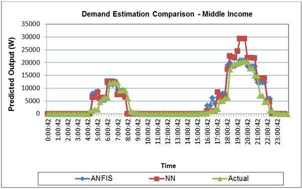
Fig. 6. Ave Daily Demand profile.
Fig. 7. ANFIS / NN Demand correlation.
Fig. 8. Morning Standard / Peak Period.
Fig. 9. Evening Peak period Demand.
6. Conclusion
Adept estimation of load profiles (lighting) is crucial for demand side management and implementation of / proposed energy efficient project across board. In development of such model, the behavioural pattern of the environment and income earning (social status) will be essential. The computational intelligence ANFIS & NN-based models based on three factors namely natural light, income and occupancy (active) were developed in the Matlab V7.10.0499 (R2010a) environment. The performance of the ANFIS-based model was better than the NN-based model as shown by the result obtained and the deduction from the statistical analysis such as
• ANFIS-based model showed the ability to learn, extracts pattern much more accurately and estimate accordingly. This is notable from the load profile output. For instance, NN-based model predicted quite low (7.15 am – 7.30 am) in the morning standard/ peak period and much higher (7.15 pm – 7.45 pm) for evening peak periods demand (Figures 8 and 9). These periods are very vital in Power Utility distribution planning (DSM) and energy efficient retrofit program in the residential sector.
• The ability to reasonable analyze / attribute values taking into consideration factors or element for various intervals instead of only identifying constant or consistent numerals to predict output as exemplified in Fig 7 by NN-based model.
• The inference attribute of the model based on characterization factors makes it a better lighting predictor resource tool thereby enhancing energy managers, measurement and verification specialists’ etc evaluation and lighting profile development.
• The study has shown that breakdown of income grouping is an essential factor that will enhance the lighting load prediction accuracy going by the result obtained from the income group and its breakdown into groupings (EM & RM)
• Based on the results obtained from the study, it can be construed that the ANFIS model is a better modelling tool for the estimation / prediction of lighting load demand profile.
Acknowledgements
This work is based on the research supported in part by the Department of Higher Education and Training Research Department Grant (DHET) RDG) and Tshwane University of Technology (TUT), South Africa.
References
- Pike Research, 2010.Energy Efficient Lighting for Commercial Markets.
- M.Stokes, M.Rylatt, and K. Lomas, A simple model of domestic lighting demand, Energy & Buildings; Vol.36: 103-116, 2004.
- S.L. Wong, K.W. Kevin, and N.T. Lam,Artificial neural networks for energy analysis of office buildings with daylighting, Applied Energy, Vol.87: 551-537, 2010.
- R. Frackowiak, and Tomczykowski, J.,Modeling of the household lighting-related load, International Journal of Electrical Power and Energy Systems,Vol.29:580-588, 2007.
- M. Aydinalp, V.I. Ugursal and A.S. Fung,Modeling of the appliance, lighting, and space-cooling energy consumptions in the residential sector using neural networks, Applied Energy, Vol.71:87-110, 2002.
- S. Zhu, J. Wang, W. Zhao and J. Wang, A seasonal hybrid procedure for electricity demand forecasting in China, Applied Energy, Vol.88:3807–3815, June 2011.
- P. Chang, Y. Fan and J. Lin, Monthly electricity demand forecasting based on weighted evolving fuzzy neural network approach, International Journal of Electrical Power and Energy Systems, Vol.33:17-27, 2011.
- D. Bourgeois, C. Reinhart,& I. Macdonald,Adding advanced behavioural models in whole building energy simulation: A study on the total energy impact of manual and automated lighting control, Energy & Buildings, Vol.38:814–823, 2006.
- I. Apolinário, C. Correia De Barros, H. Coutinho,L. Ferreira, B. Madeira, P. Oliveira,A. Tavares, A.Trindade, P.Verdelho,Behavioural Factors’ Influence on Energy Savings,20th International Conference on Electricity Distribution, Prague, 2009, pp. 8-11.
- Gago Eclalia Jadraque, Garcia Javier Ordonez & Estrella Antonio Espin,Development of energy model for residential sector: Electricity consumption in Andalusia, Spain, Energy & Buildings, Vol.43:1315-1321, Jan. 2011.
- I. Richardson, M.Thomson, D.Infeild and A. Delahunty,Domestic lighting: A high-resolution energy demand model.Energy & Buildings,Vol. 41: 781-789, May 2009.
- C. Engelbrecht, C.A. Van Der Merwe, L.J. Grobler, E.L. Meyer,M.Simon, and D. Van Es,Do CFL Programs Have an impact on Supply,Domestic Use of Energy Conference 2008, March 17-20.
- J.O. Folorunsho, E.O. Igunsi, M.B. Mu’azu, and S. Garba, S.,Application of adaptive Neuro Fuzzy inference System (Anfis) in River Kaduna Discharge Forecasting, Research Journal of applied Sciences, engineering and Technology, Vol.4(21):4275–4283, November. 2012.
- S.R. Sibendu,Design of adaptive neuro - fuzzy inference system for predicting surface roughness in turning operation, Journal of Scientific & Industrial Research, Vol. 64: 653–659, Sept.2005.
- F. Chang, and Y. Chang, Adaptive neuro-fuzzy system for prediction of Water level in reservoir,’ Advances in Water Resources, Vol.29:1-10, 2006.
- M. Firat, and M. Gungor, M. River flow estimation using adaptive neuro fuzzy inference system, Mathematics and Computer in simulations, Vol.75: 87-96, 2007.
- L. Ying, and M. Pan,Using adaptive network based fuzzy inference system to forecast regional electricity loads, Energy Conversion and Management, Vol.49:205–211, 2008.
- Yun, Z., Quan, Z., Caixin, S., Shaolan, L, Yuming, L., and Yang, S. RBF Neural Network and ANFIS – Based Short – Term Load Forecasting Approach in Real – Time Price Environment. IEEE T Power Syst,Vol. 23(3):853–858, Aug. 2008.
- J.R. Jang, ANFIS: Adaptive – Network – Based Fuzzy Inference System, IEEE Transactions on Systems, Man and Cybernetics, Vol.23 (3) 665–684, May / June 1993.
- J. Page, D. Robinson, and Jl. Scartezzini, Stochastic Simulation of Occupant Presence and Behaviour in Buildings. Building Simulation 2007: 757-764.
- Popoola, O., Munda, J., & Mpanda, A. "Residential Lighting load Profile Modelling. Energy and Buildings, 2015; Vol. 90: 29-40.